Tutorial#
This section contains a short tutorial that describes how to get ready
to use the framework. It assumes that you have already installed the
litebird_sim framework; refer to Installation.
For a nice and exhaustive example on how to use the framework in the
LiteBIRD case see the example notebook.
A «Hello world» example#
In this section we assume that you are running these command
interactively, either using the REPL (python or IPython are both
fine) or a Jupyter notebook.
The first thing to do is to create a folder where you will write your script. The LiteBIRD Simulation Framework is a library, and thus it should be listed as one of the dependencies of your project. It’s better to use virtual environments, so that dependencies are properly tracked:
python -m virtualenv ./lbs_tutorial_venv
source lbs_tutorial_venv/bin/activate
The last line of code might vary, depending on the Operating System and the shell you are using; refer to the Python documentation for more information.
Once you have activated the virtual environment, you should install
the LiteBIRD Simulation Framework. As it is registered on PyPI, it’s just a matter of
calling pip:
pip install litebird_sim
To ensure reproducibility of your results, it is good to keep track of
the version numbers used by your program. If you are developing with uv
(recommended for LiteBIRD Simulation Framework development), uv automatically
creates a uv.lock file that pins exact versions:
# With uv (recommended for development)
uv sync  # This creates/updates uv.lock automatically
Alternatively, if using pip, you can create a requirements.txt file:
pip freeze > requirements.txt
(If you use a Version Control System like git, it is a good idea
to add uv.lock or requirements.txt to the repository.) Others will then be
able to install the same versions by using uv sync or pip install -r requirements.txt.
If you got no errors, you are ready to write your first program! To
follow an ancient tradition, we will write a «Hello world!» program.
Create a new file called my_script.py in the folder you just
created, and write the following:
# File my_script.py
import litebird_sim as lbs

print("Starting the program...")
sim = lbs.Simulation(base_path="./tut01", random_seed=12345)
sim.append_to_report("Hello, world!")
sim.flush()
print("Done!")
Surprisingly, the program did not output Hello world as you might
have expected! Instead, it created a folder, named tut01, and
wrote a few files in it:
$ ls ./tut01
report.html    report.md    sakura.css
$
Open the file report.html using your browser (e.g., firefox
tut01/report.html), and the following page will appear:

Among the many lines of text produced by the report, you can spot the presence of our «Hello, world!» message. Hurrah!
Let’s have a look at what happened. The first line imports the
litebird_sim framework; since the name is quite long, it’s
customary to shorten it to lbs:
import litebird_sim as lbs
The next interesting stuff happens when we instantiate a
Simulation object:
sim = lbs.Simulation(base_path="./tut01", random_seed=12345,)
Creating a Simulation object makes a lot of complicated
things happen behind the scenes. For example, the mandatory parameter
random_seed is used to build a hierarchy of random number generators useful for
generating noise. In this short example, the important things are
the following:
The code checks if a directory named
tut01exists; if not, it is created.An empty report is created.
The report is where the results of a simulation will be saved, and
sections can be appended to it using the method
Simulation.append_to_report(), like we did in our example:
sim.append_to_report("Hello, world!")
The report is actually written to disk only when
Simulation.flush() is called:
sim.flush()
This is the most basic usage of the Simulation class; for
more information, refer to Simulations.
In the next section, we will make something more interesting using the framework.
Interacting with the IMO#
It’s not clear why we should want to install a whole framework just to create a HTML file, no matter how nice it looks. Things begin to get interesting once we start using other facilities provided by our framework.
Simulations for real-life experiments often require to use several parameters that describe the instruments being simulated: how many detectors there are, what are their properties, etc. These information are usually kept in an Instrument MOdel database, IMO for short.
The LiteBIRD IMO is managed using InstrumentDB, a web-based database, but it can be retrieved also as a bundle of files. The LiteBIRD simulation framework seamlessy interacts with the IMO database and permits to retrieve all the parameters that describe the LiteBIRD instruments.
The simulation framework contains a IMO containing a small representation of the instruments as described in the paper *Probing cosmic inflation with the LiteBIRD cosmic microwave background polarization survey* (PTEP, 2022). We will use this small IMO in the tutorial; if you want to do some serious work, you should install your own copy of the “full” official IMO. Refer to Configuring the IMO for more information.
Our next example will use the IMO to run something more interesting:
import litebird_sim as lbs

imo = lbs.Imo(flatfile_location=lbs.PTEP_IMO_LOCATION)

sim = lbs.Simulation(base_path="./tut02", random_seed=12345)
lft_file = sim.imo.query(
    "/releases/vPTEP/satellite/LFT/instrument_info"
)
sim.append_to_report(
    "The instrument {{ name }} has {{ num }} channels.",
    name=lft_file.metadata["name"],
    num=lft_file.metadata['number_of_channels'],
)

html_report_path = sim.flush()
print(f"Done, the report has been saved in file {html_report_path.name}")
Done, the report has been saved in file report.html
Let’s dig into the code of the example. The first line looks almost the same as in the previous example:
# Previous example
sim = lbs.Simulation(base_path="./tut01", random_seed=12345)

# This example
sim = lbs.Simulation(base_path="./tut02", random_seed=12345)
Yet a big difference went unnoticed: since you configured the IMO
using the install_imo module, the Simulation class
managed to read the database contents and initialize a set of member
variables. This is why we have been able to write the next line:
lft_file = sim.imo.query(
    "/releases/vPTEP/satellite/LFT/instrument_info"
)
Although the parameter looks like a path to some file, it is a
reference to a bit of information in the IMO; specifically, a set of
parameters characterizing the instrument LFT (Low Frequency
Telescope). This call retrieves the parameters and returns a
DataFile object, which contains the information in its
metadata field. These are used to fill the report:
sim.append_to_report(
    "The instrument {{ name }} has {{ num }} channels.",
    name=lft_file.metadata["name"],
    num=lft_file.metadata['number_of_channels'],
)
The code should be self-evident: the keywords name and num are
used in the text to put some actual values within the placeholders
{{ … }}. This is the syntax used by Jinja2, a powerful
templating library.
The last lines write the report to disk and return the path to the HTML file:
html_report_path = sim.flush()
print(f"Done, the report has been saved in file {html_report_path.name}")
This example showed you how to retrieve information from the IMO and
introduced some features of the method
Simulation.append_to_report(). To learn a bit more about the
the IMO, read The IMo; for reporting facilities, read
Creating reports.
Creating a coverage map#
We’re now moving to something more «astrophysical»: we will write a program that computes the sky coverage of a scanning strategy over some time.
The code is complex because it uses several concepts explained in the section Scanning strategy; in fact, this example is very similar to the one shown in that section. It’s not needed that you understand everything, just have a look at the code that generates the report:
import litebird_sim as lbs
import healpy, numpy as np
import matplotlib.pylab as plt
import astropy.units as u
imo = lbs.Imo(flatfile_location=lbs.PTEP_IMO_LOCATION)
sim = lbs.Simulation(
base_path="./tut04",
name="Simulation tutorial",
start_time=0,
duration_s=86400.,
random_seed=12345,
imo=imo,
)
sim.set_scanning_strategy(
scanning_strategy=lbs.SpinningScanningStrategy.from_imo(
imo=imo,
url="/releases/vPTEP/satellite/scanning_parameters",
),
)
sim.set_instrument(
lbs.InstrumentInfo.from_imo(
imo=imo,
url="/releases/vPTEP/satellite/LFT/instrument_info",
),
)
sim.set_hwp(lbs.IdealHWP(ang_speed_radpsec=0.1))
# It is entirely possible to mix up definitions taken from
# the IMO with hand-made objects. In this example, we create
# a mock detector instead of reading one from the PTEP IMO.
sim.create_observations(
detectors=lbs.DetectorInfo(name="foo", sampling_rate_hz=10),
)
sim.prepare_pointings()
for cur_obs in sim.observations:
# We use `_` to ignore the HWP angle
cur_pointings, _ = cur_obs.get_pointings(0)
nside = 64
pixidx = healpy.ang2pix(
nside,
cur_pointings[:, 0],
cur_pointings[:, 1],
)
m = np.zeros(healpy.nside2npix(nside))
m[pixidx] = 1
healpy.mollview(m)
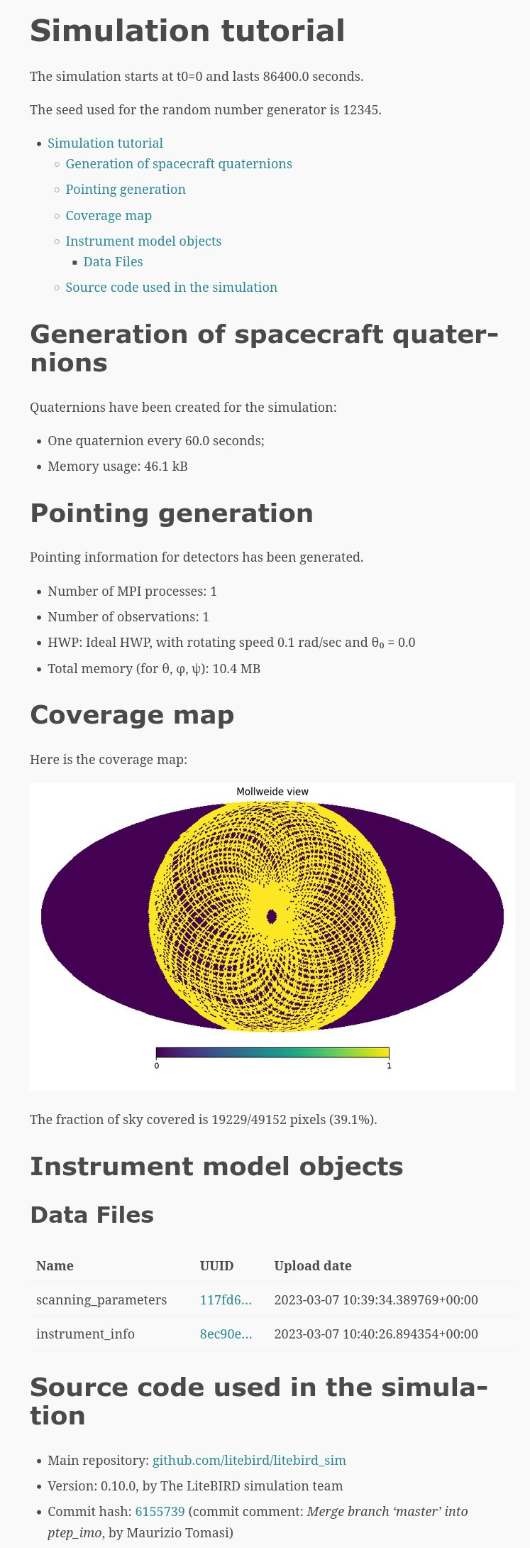
sim.append_to_report("""
## Coverage map
Here is the coverage map:

The fraction of sky covered is {{ seen }}/{{ total }} pixels
({{ "%.1f" | format(percentage) }}%).
""",
figures=[(plt.gcf(), "coverage_map.png")],
seen=len(m[m > 0]),
total=len(m),
percentage=100.0 * len(m[m > 0]) / len(m),
)
sim.flush()
This example is interesting because it shows how to interface Healpy with the report-generation facilities provided by our framework. As explained in Scanning strategy, the code above does the following things:
It sets the scanning strategy, triggering the computation of set of quaternions that encode the orientation of the spacecraft for the whole duration of the simulation (86,400 seconds, that is one day);
It creates an instance of the class
InstrumentInfoand it registers them using the methodSimulation.set_instrument();It instantiates a new class that represents an ideal Half-wave Plate (HWP);
It sets the detectors to be simulated and allocates the TODs through the call to
Simulation.create_observations();It computes the quaternions needed to compute the actual pointings through the call to
Simulation.prepare_pointings();It produces a coverage map by setting to 1 all those pixels that are visited by the directions encoded in the pointing information matrix. To do this, it iterates over all the instances of the class
Observationin theSimulationobject. (In this simple example, there is only oneObservation, but in more complex examples there can be many of them.) For eachObservation, it uses the methodObservation.get_pointings()to compute the pointing information for that observation.The objects that were read from IMO are properly listed in the report.
If you run the example, you will see that the folder tut04 will be
populated with the following files:
$ ls tut04
coverage_map.png  report.html  report.md  sakura.css
$
A new file has appeared: coverage_map.png. If you open the file
report.html, you will see that the map has been included in the
report:
Creating a signal plus noise timeline#
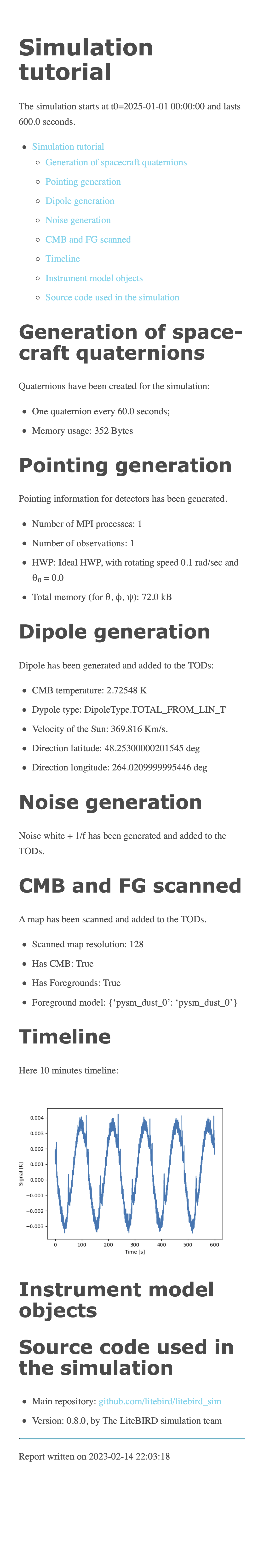
Here we generate a 10 minutes timeline which contains dipole, cmb signal,
galactic dust, and correlated noise. For the noise, we use the random
number generator provided by the Simulation and seeded with
random_seed:
import litebird_sim as lbs
import healpy, numpy as np
import matplotlib.pylab as plt
from astropy import units, time
sim = lbs.Simulation(
base_path="./tut05",
name="Simulation tutorial",
start_time=time.Time("2025-01-01T00:00:00"),
duration_s=10 * units.minute.to("s"),
random_seed=12345,
)
sim.set_scanning_strategy(
scanning_strategy=lbs.SpinningScanningStrategy(
spin_sun_angle_rad=np.deg2rad(30), # CORE-specific parameter
spin_rate_hz=0.5 / 60, # Ditto
precession_rate_hz=1.0 / (4 * units.day).to("s").value,
)
)
sim.set_instrument(
lbs.InstrumentInfo(
name="core",
spin_boresight_angle_rad=np.deg2rad(65),
),
)
sim.set_hwp(lbs.IdealHWP(ang_speed_radpsec=0.1))
detector = lbs.DetectorInfo(
name="foo",
sampling_rate_hz=10.0,
bandcenter_ghz = 200.0,
net_ukrts = 50.0,
fknee_mhz = 20.0,
fmin_hz = 1e-05,
alpha=1.0,
)
sky_params = lbs.SkyGenerationParams(
nside=128,
make_cmb=True,
make_fg=True,
fg_models=["d0"],
)
sky_gen = lbs.SkyGenerator(
parameters=sky_params,
detectors=detector,
)
maps = sky_gen.execute()
sim.create_observations(
detectors=detector,
)
sim.prepare_pointings()
sim.add_dipole()
sim.add_noise()
sim.fill_tods(maps=maps)
times = sim.observations[0].get_times() - sim.observations[0].start_time.cxcsec
plt.plot(times,sim.observations[0].tod[0,:])
plt.xlabel("Time [s]")
plt.ylabel("Signal [K]")
sim.append_to_report("""
## Timeline
Here 10 minutes timeline:

""",
figures=[(plt.gcf(), "timeline.png")],
)
sim.flush()
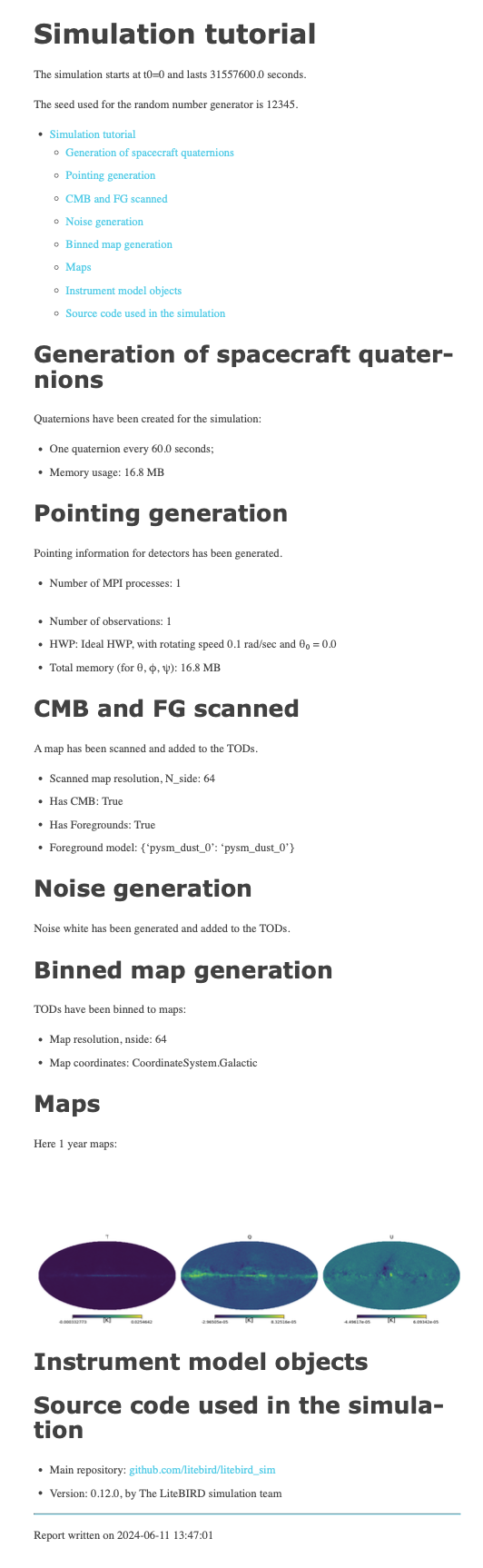
Creating a signal plus noise timeline#
Here we generate a 1 year timeline which contains cmb signal, galactic dust, and white noise. The we bin the timeline in a map.
import litebird_sim as lbs
import numpy as np
import matplotlib.pylab as plt
import healpy as hp
from astropy import units, time
sim = lbs.Simulation(
base_path="./tut06",
name="Simulation tutorial",
start_time=0,
duration_s=1 * units.year.to("s"),
random_seed=12345,
)
nside = 64
sim.set_scanning_strategy(
scanning_strategy=lbs.SpinningScanningStrategy(
spin_sun_angle_rad=np.deg2rad(30), # CORE-specific parameter
spin_rate_hz=0.5 / 60, # Ditto
precession_rate_hz=1.0 / (4 * units.day).to("s").value,
)
)
sim.set_instrument(
lbs.InstrumentInfo(
name="core",
spin_boresight_angle_rad=np.deg2rad(65),
),
)
sim.set_hwp(lbs.IdealHWP(ang_speed_radpsec=0.1))
detector = lbs.DetectorInfo(
name="foo",
sampling_rate_hz=3.0,
bandcenter_ghz = 150.0,
net_ukrts = 50.0,
)
sky_params = lbs.SkyGenerationParams(
nside=nside,
make_cmb=True,
make_fg=True,
fg_models=["d0"],
)
sky_gen = lbs.SkyGenerator(
parameters=sky_params,
detectors=detector,
)
maps = sky_gen.execute()
sim.create_observations(
detectors=detector,
)
sim.prepare_pointings()
sim.fill_tods(maps)
sim.add_noise(noise_type="white")
binner_results = sim.make_binned_map(nside=nside)
binned = binner_results.binned_map
plt.figure(figsize=(15, 3.2))
hp.mollview(binned[0], sub=131, title="T", unit=r"[K]")
hp.mollview(binned[1], sub=132, title="Q", unit=r"[K]")
hp.mollview(binned[2], sub=133, title="U", unit=r"[K]")
sim.append_to_report("""
## Maps
Here 1 year maps:

""",
figures=[(plt.gcf(), "maps.png")],
)
sim.flush()
The elements shown in these tutorials should allow you to generate more complex scripts. The next sections detail the features of the framework in greater detail.