Dipole anisotropy#
The LiteBIRD Simulation Framework provides tools to simulate the signal associated with the relative velocity between the rest frame of the spacecraft with respect to the CMB. The motion of the spacecraft in the rest frame of the CMB is the composition of several components:
The motion of the spacecraft around L2;
The motion of the L2 point in the Ecliptic plane;
The motion of the Solar System around the Galactic Centre;
The motion of the Milky Way.
Components 1 and 2 are simulated by the LiteBIRD Simulation Framework using appropriate motion models, while components 3 and 4 are included using the Sun velocity derived by the solar dipole measured by the Planck satellite.
The motion of the spacecraft around L2 is modelled using a Lissajous
orbit similar to what was used for the WMAP experiment
[1], and it is encoded using the
SpacecraftOrbit class.
Position and velocity of the spacecraft#
The class SpacecraftOrbit describes the orbit of the
LiteBIRD spacecraft with respect to the Barycentric Ecliptic Reference
Frame and the motion of the Barycentric Ecliptic Reference Frame with
respect to the CMB; this class is necessary because the class
ScanningStrategy (see the chapter Scanning strategy)
only models the direction each instrument is looking at but knows
nothing about the velocity of the spacecraft itself.
The class SpacecraftOrbit is a dataclass that can initialize
its members to sensible default values taken from the literature. As
the LiteBIRD orbit around L2 is not fixed yet, the code assumes a
WMAP-like Lissajous orbit, [1]. For the Sun
velocity it assumes Planck 2018 solar dipole
[7].
To compute the position/velocity of the spacecraft, you call
spacecraft_pos_and_vel(); it requires either a period or an
Observation object, and it returns an instance of the class
SpacecraftPositionAndVelocity:
import litebird_sim as lbs
from astropy.time import Time

orbit = lbs.SpacecraftOrbit(start_time=Time("2023-01-01"))
posvel = lbs.spacecraft_pos_and_vel(
    orbit,
    start_time=orbit.start_time,
    time_span_s=86_400.0,  # One day
    delta_time_s=3600.0    # One hour
)

print(posvel)
SpacecraftPositionAndVelocity(start_time=2023-01-01 00:00:00.000, time_span_s=86400.0, nsamples=25)
The output of the script shows that 25 «samples» have been computed;
this means that the posvel variable holds information about 25
position/velocity pairs evenly spaced between 2023-01-01 and
2023-01-02: one at midnight, one at 1:00, etc., till midnight
2023-01-02. The SpacecraftPositionAndVelocity class keeps
the table with the positions and the velocities in the fields
positions_km and velocities_km_s, respectively, which are
arrays of shape (nsamples, 3).
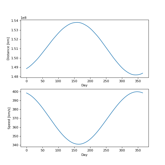
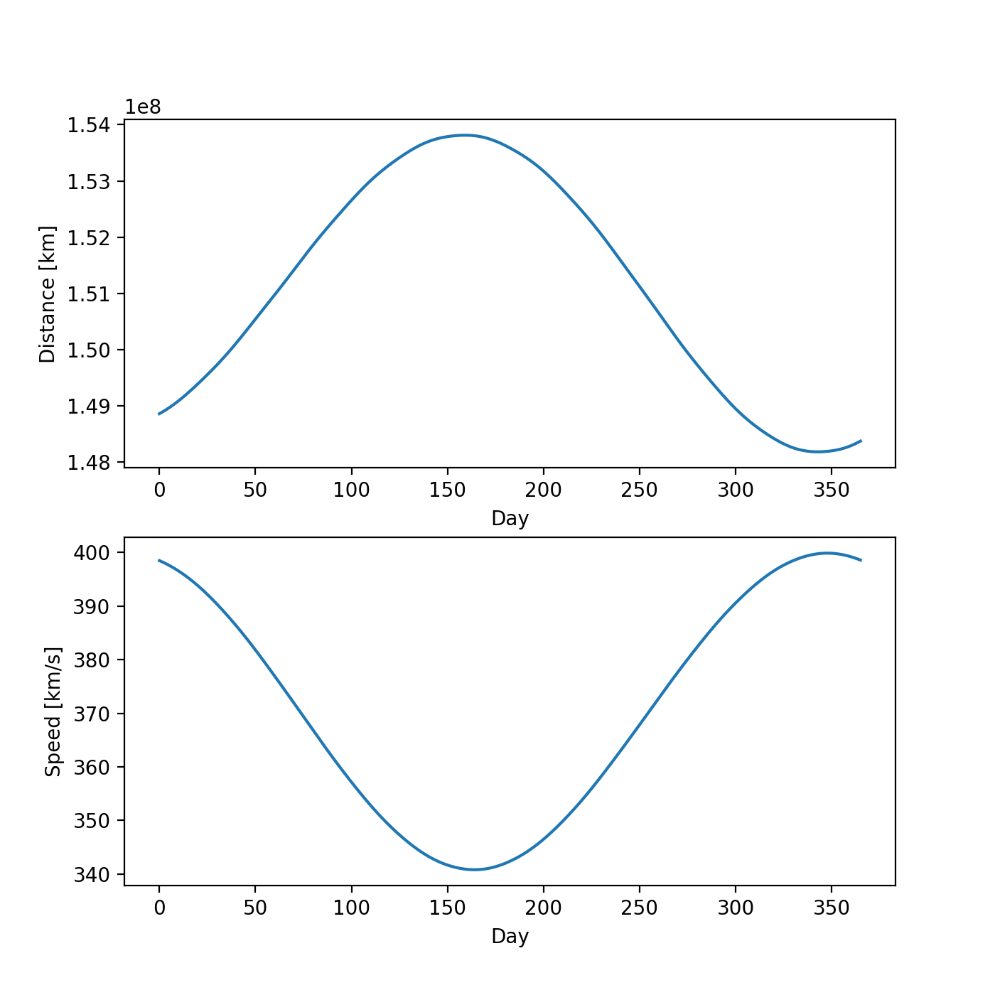
Here is a slightly more complex example that shows how to plot the distance between the spacecraft and the Sun as a function of time and speed. The latter quantity is, of course, most relevant when computing the CMB dipole.
import numpy as np
import litebird_sim as lbs
from astropy.time import Time
import matplotlib.pylab as plt

orbit = lbs.SpacecraftOrbit(start_time=Time("2023-01-01"))

posvel = lbs.spacecraft_pos_and_vel(
    orbit,
    start_time=orbit.start_time,
    time_span_s=3.15e7,  # One year
    delta_time_s=86_400.0,  # One day
)

# posvel.positions_km is a N×3 array containing the XYZ position
# of the spacecraft calculated every day for one year. We compute
# the modulus of the position, which is of course the
# Sun-LiteBIRD distance.
sun_distance_km = np.linalg.norm(posvel.positions_km, axis=1)

# We do the same with the velocities
speed_km_s = np.linalg.norm(posvel.velocities_km_s, axis=1)

# Plot distance and speed as functions of time
_, ax = plt.subplots(nrows=2, ncols=1, figsize=(7, 7))

ax[0].plot(sun_distance_km)
ax[0].set_xlabel("Day")
ax[0].set_ylabel("Distance [km]")

ax[1].plot(speed_km_s)
ax[1].set_xlabel("Day")
ax[1].set_ylabel("Speed [km/s]")
(Source code, png, hires.png, pdf)

Computing the dipole#
The CMB dipole is caused by a Doppler shift of the frequencies observed while looking at the CMB blackbody spectrum. In thermodynamic temperature units the observed temperature along the direction \(\hat n\) is
where \(T_0\) is the temperature in the rest frame of the CMB, \(\vec \beta = \vec v / c\) is the dimensionless velocity vector, \(\hat n\) is the direction of the line of sight, and \(\gamma = \bigl(1 - \vec\beta \cdot \vec\beta\bigr)^{-1/2}\). The TOD routines add the temperature fluctuation \(\Delta T = T(\vec\beta,\hat n) - T_0\).
However, CMB experiments usually employ the linear thermodynamic temperature definition, where temperature differences \(\Delta_1 T\) are related to the actual temperature difference \(\Delta T\) by the relation
where \(x = h \nu / k_B T\),
and \(\mathrm{BB}(\nu, T)\) is the spectral radiance of a black-body according to Planck’s law:
There is no numerical issue in computing the complete formula, but
series approximations are often useful when separating the dipole,
quadrupole, and octupole contributions. The LiteBIRD Simulation
Framework selects the model through DipoleType:
Type |
Formula |
Notes |
|---|---|---|
|
\(T_0 b\) |
First order, where \(b=\vec\beta\cdot\hat n\). |
|
\(T_0\left(b + b^2\right)\) |
Thermodynamic expansion to second order. The monopole \(-T_0\beta^2/2\) is omitted. |
|
\(T_0\left(b + b^2 + b^3\right)\) |
Thermodynamic expansion to third order, again omitting monopole terms from the \(\gamma\) factor. |
|
\(T_0/\left[\gamma(1-b)\right] - T_0\) |
Exact thermodynamic-temperature formula. |
|
\(T_0\left[b + q(x)b^2\right]\) |
Second-order expansion in linearized thermodynamic units. |
|
\(T_0\left[b + q(x)b^2 + r(x)b^3\right]\) |
Third-order expansion in linearized thermodynamic units. |
|
Full expression from (2) |
The default model, typically used by CMB experiments. |
The frequency-dependent weights in the linearized expansions are
Beam convolution is not a separate DipoleType; it is enabled
by passing beam S-parameters to add_dipole() (the s_params
keyword) or by setting apply_convolution=True on
add_dipole_to_observations(), as described below.
You can add the dipole signal to an existing TOD through the
function add_dipole_to_observations(), as the following example
shows:
from astropy.time import Time
import numpy as np
import litebird_sim as lbs
import matplotlib.pylab as plt

start_time = Time("2022-01-01")
time_span_s = 120.0  # Two minutes
sampling_hz = 20

sim = lbs.Simulation(start_time=start_time, duration_s=time_span_s, random_seed=12345)

# We pick a simple scanning strategy where the spin axis is aligned
# with the Sun-Earth axis, and the spacecraft spins once every minute
sim.set_scanning_strategy(
    lbs.SpinningScanningStrategy(
        spin_sun_angle_rad=np.deg2rad(0),
        precession_rate_hz=0,
        spin_rate_hz=1 / 60,
        start_time=start_time,
    ),
    delta_time_s=5.0,
)

# We simulate an instrument whose boresight is perpendicular to
# the spin axis.
sim.set_instrument(
    lbs.InstrumentInfo(
        boresight_rotangle_rad=0.0,
        spin_boresight_angle_rad=np.deg2rad(90),
        spin_rotangle_rad=np.deg2rad(75),
    )
)

# A simple detector looking along the boresight direction
det = lbs.DetectorInfo(
    name="Boresight_detector",
    sampling_rate_hz=sampling_hz,
    bandcenter_ghz=100.0,
)

(obs,) = sim.create_observations(detectors=[det])

sim.prepare_pointings()

# Simulate the orbit of the spacecraft and compute positions and
# velocities
orbit = lbs.SpacecraftOrbit(obs.start_time)
pos_vel = lbs.spacecraft_pos_and_vel(orbit, obs, delta_time_s=60.0)

t = obs.get_times()
t -= t[0]  # Make `t` start from zero

# Create two plots: the first shows the full two-minute time span, and
# the second one shows a zoom over the very first points of the TOD.
_, axes = plt.subplots(nrows=2, ncols=1, figsize=(10, 12))

# Make a plot of the TOD using all the dipole types. Beam convolution is
# controlled by the apply_convolution keyword, not by a separate DipoleType.
for type_idx, dipole_type in enumerate(lbs.DipoleType):
    obs.tod[0][:] = 0  # Reset the TOD
    lbs.add_dipole_to_observations(obs, pos_vel, dipole_type=dipole_type)

    axes[0].plot(t, obs.tod[0], label=str(dipole_type))
    axes[1].plot(t[0:20], obs.tod[0][0:20], label=str(dipole_type))

axes[0].set_xlabel("Time [s]")
axes[0].set_ylabel("Signal [K]")
axes[1].set_xlabel("Time [s]")
axes[1].set_ylabel("Signal [K]")
axes[1].legend()
The example plots two minutes of a simulated timeline for a very simple instrument, and it zooms over the very first points to show that there is indeed some difference in the estimate provided by each method.
Beam-convolved dipole#
When a real instrument observes the CMB, its response is spread over the full 4π sky by the beam, including far sidelobes. This changes the dipole template used for photometric calibration. The implementation follows the moment expansion in Appendix C of the Planck NPIPE paper [8].
For the frequency-dependent linearized expansion the sky template is
which corresponds to DipoleType.QUADRATIC_FROM_LIN_T.
A detector with beam pattern \(B(\hat n)\) (normalized so that \(\int B(\hat n)\,d\Omega = 1\)) observes a beam-convolved signal
Expanding in Cartesian components and rotating the velocity into the beam frame (boresight along \(\hat z\)), the integral reduces to a dot product with pre-computed beam moments (Eq. C.5 of NPIPE):
where \(\boldsymbol\beta\) is the velocity in the beam frame and the S-parameters are
These integrals are computed once per detector from the full 4π
beam harmonics and then reused for every TOD sample. Convolution by
moment expansion is the only supported way to beam-convolve the dipole.
It supports the polynomial-expansion models DipoleType.LINEAR,
DipoleType.QUADRATIC_EXACT, DipoleType.CUBIC_EXACT,
DipoleType.QUADRATIC_FROM_LIN_T, and DipoleType.CUBIC_FROM_LIN_T.
The total-formula models DipoleType.TOTAL_EXACT and
DipoleType.TOTAL_FROM_LIN_T are not supported under convolution.
Computing S-parameters#
Given beam spherical harmonics in the beam frame (boresight at the
north pole), use BeamSParams.from_beam_alm():
import numpy as np
import litebird_sim as lbs

beam_alm = lbs.gauss_beam_to_alm(
    lmax=64,
    mmax=64,
    fwhm_rad=np.deg2rad(30.0 / 60.0),
    psi_pol_rad=None,
)
s_params = lbs.BeamSParams.from_beam_alm(beam_alm)
The result is a BeamSParams object holding the 3-element
vector s_vec, the 3×3 matrix s_mat, and the 3×3×3 tensor
s_ten. If a polarized beam object is provided, only its temperature
component is used for the scalar dipole convolution.
For a circularly symmetric beam, \(S_x = S_y = 0\) and \(S_{xy} = S_{xz} = S_{yz} = 0\) by symmetry, so only \(S_z\), \(S_{xx} = S_{yy}\), and \(S_{zz}\) are non-zero. As a sanity check, \(S_{xx} + S_{yy} + S_{zz} = 1\) (trace equals the beam normalisation).
Adding a convolved dipole#
For the low-level add_dipole(), compute the beam S-parameters
with BeamSParams.from_beam_alm() and pass them via s_params.
The pointing matrices must include the \(\psi\) column, with shape
(n_det, n_samples, 3). Choose any polynomial-expansion
DipoleType; the example below uses
DipoleType.QUADRATIC_FROM_LIN_T:
import litebird_sim as lbs
import numpy as np

n_samples = 3
pointings = np.deg2rad(
    np.array([[[90, 0, 0], [90, 90, 0], [90, 180, 0]]], dtype=float)
)
velocity = np.tile([300.0, 0.0, 0.0], (n_samples, 1))
tod = np.zeros((1, n_samples))

beam_alm = lbs.gauss_beam_to_alm(
    lmax=32,
    mmax=32,
    fwhm_rad=np.deg2rad(30.0),
    psi_pol_rad=None,
)
s_params = lbs.BeamSParams.from_beam_alm(beam_alm)

lbs.add_dipole(
    tod,
    pointings,
    velocity,
    t_cmb_k=lbs.T_CMB_K,
    frequency_ghz=np.array([100.0]),
    dipole_type=lbs.DipoleType.QUADRATIC_FROM_LIN_T,
    s_params=s_params,
)
For more than one detector, s_params can be a single
BeamSParams object reused for all detectors, or a dictionary
keyed by detector index strings ("0", "1", …). The
observation-oriented add_dipole_to_observations() instead takes
beam harmonics directly: set apply_convolution=True and pass
beam_alms (or store them on the observation’s blms attribute),
and it computes the S-parameters per detector for you. If beam_alms
is a dictionary, its keys must be detector or channel names (not
index strings), consistent with add_convolved_sky().
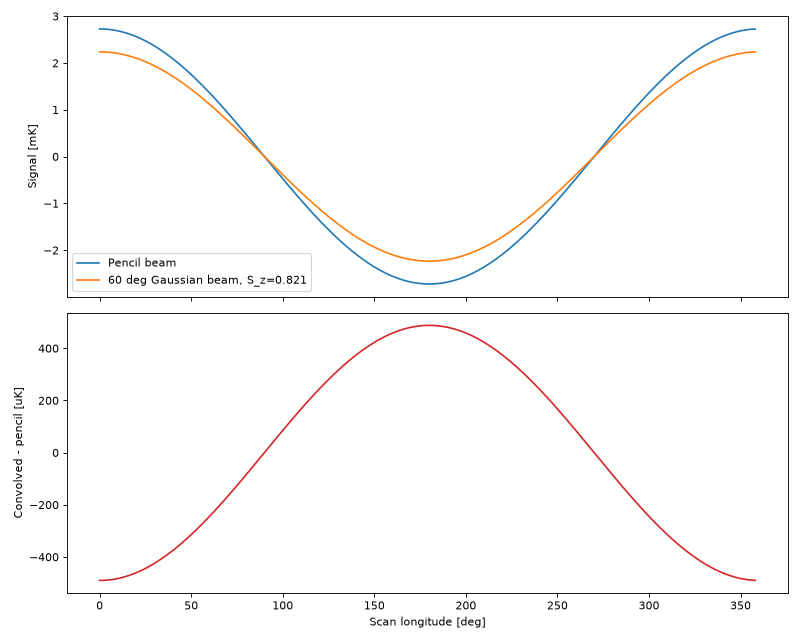
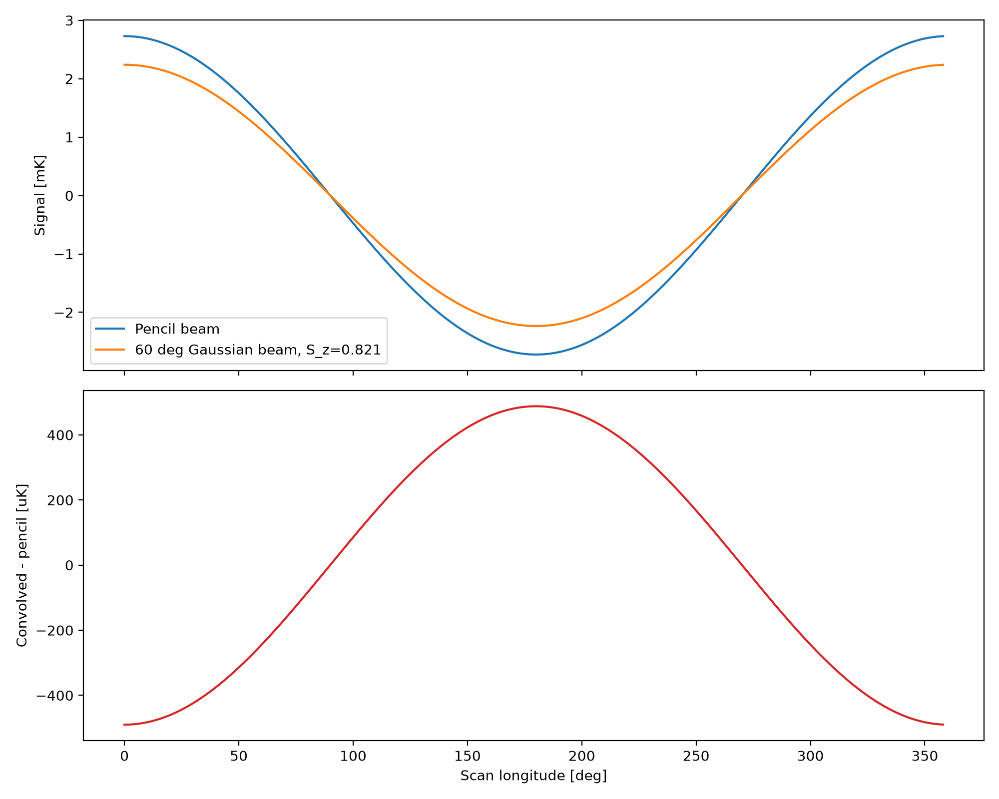
The following plot compares the ordinary
DipoleType.QUADRATIC_FROM_LIN_T dipole with the same model after
convolution with a wide Gaussian beam. The upper panel shows both
signals and the lower panel shows the difference, which is dominated by
the beam suppression of the dipole amplitude.
import matplotlib.pylab as plt
import numpy as np

import litebird_sim as lbs


n_samples = 180
phi = np.linspace(0.0, 2.0 * np.pi, n_samples, endpoint=False)

pointings = np.zeros((1, n_samples, 3))
pointings[0, :, 0] = np.pi / 2.0  # Equatorial scan
pointings[0, :, 1] = phi
pointings[0, :, 2] = 0.0

beta = 1.0e-3
velocity = np.tile([lbs.C_LIGHT_KM_OVER_S * beta, 0.0, 0.0], (n_samples, 1))
frequency_ghz = np.array([100.0])

beam_alm = lbs.gauss_beam_to_alm(
    lmax=64,
    mmax=64,
    fwhm_rad=np.deg2rad(60.0),
    psi_pol_rad=None,
)
s_params = lbs.BeamSParams.from_beam_alm(beam_alm)

tod_pencil = np.zeros((1, n_samples))
lbs.add_dipole(
    tod_pencil,
    pointings,
    velocity,
    t_cmb_k=lbs.T_CMB_K,
    frequency_ghz=frequency_ghz,
    dipole_type=lbs.DipoleType.QUADRATIC_FROM_LIN_T,
)

tod_convolved = np.zeros((1, n_samples))
lbs.add_dipole(
    tod_convolved,
    pointings,
    velocity,
    t_cmb_k=lbs.T_CMB_K,
    frequency_ghz=frequency_ghz,
    dipole_type=lbs.DipoleType.QUADRATIC_FROM_LIN_T,
    s_params=s_params,
)

scan_angle_deg = np.rad2deg(phi)
diff_uk = (tod_convolved[0] - tod_pencil[0]) * 1.0e6

_, axes = plt.subplots(nrows=2, ncols=1, figsize=(10, 8), sharex=True)

axes[0].plot(scan_angle_deg, tod_pencil[0] * 1.0e3, label="Pencil beam")
axes[0].plot(
    scan_angle_deg,
    tod_convolved[0] * 1.0e3,
    label=f"60 deg Gaussian beam, S_z={s_params.s_vec[2]:.3f}",
)
axes[0].set_ylabel("Signal [mK]")
axes[0].legend()

axes[1].plot(scan_angle_deg, diff_uk, color="tab:red")
axes[1].set_xlabel("Scan longitude [deg]")
axes[1].set_ylabel("Convolved - pencil [uK]")

plt.tight_layout()
(Source code, png, hires.png, pdf)

Interpretation of the S-parameters#
Beam |
S-parameters |
|---|---|
Perfect pencil (δ at ẑ) |
|
Isotropic (uniform 4π) |
|
Symmetric Gaussian (narrow) |
|
For the pencil beam the formula reduces to
(3), so the convolved result is identical to
QUADRATIC_FROM_LIN_T. A real beam with significant
sidelobes will have \(S_z < 1\) and \(S_{xx} = S_{yy} > 0\),
which suppresses the dipole amplitude and introduces a small
pointing-independent offset (from \(S_{ij}\beta_i\beta_j\)).
Methods of class simulation#
The class Simulation provides two simple functions that compute
position and velocity of the spacecraft Simulation.compute_pos_and_vel(),
and add the solar and orbital dipole to all the observations of a given
simulation Simulation.add_dipole().
import litebird_sim as lbs
from astropy.time import Time
import numpy as np

start_time = Time("2025-01-01")
time_span_s = 1000.0
sampling_hz = 10.0

sim = lbs.Simulation(
    start_time=start_time,
    duration_s=time_span_s,
    random_seed=12345,
)

# We pick a simple scanning strategy where the spin axis is aligned
# with the Sun-Earth axis, and the spacecraft spins once every minute
sim.set_scanning_strategy(
    lbs.SpinningScanningStrategy(
        spin_sun_angle_rad=np.deg2rad(0),
        precession_rate_hz=0,
        spin_rate_hz=1 / 60,
        start_time=start_time,
    ),
    delta_time_s=5.0,
 )

# We simulate an instrument whose boresight is perpendicular to
# the spin axis.
sim.set_instrument(
    lbs.InstrumentInfo(
        boresight_rotangle_rad=0.0,
        spin_boresight_angle_rad=np.deg2rad(90),
        spin_rotangle_rad=np.deg2rad(75),
    )
)

# A simple detector looking along the boresight direction
det = lbs.DetectorInfo(
    name="Boresight_detector",
    sampling_rate_hz=sampling_hz,
    bandcenter_ghz=100.0,
)

sim.create_observations(detectors=det)

sim.prepare_pointings()

sim.compute_pos_and_vel()

sim.add_dipole()

for i in range(5):
    print(f"{sim.observations[0].tod[0][i]:.5e}")
3.44963e-03
3.45207e-03
3.45413e-03
3.45582e-03
3.45712e-03
Note that even if Simulation.compute_pos_and_vel() is not explicitly
invoked, Simulation.add_dipole() takes care of that internally initializing
SpacecraftOrbit and computing positions and velocities.
API reference#
- class litebird_sim.spacecraft.SpacecraftOrbit(start_time: Time, earth_l2_distance_km: float = 1496509.30522, radius1_km: float = 244450.0, radius2_km: float = 137388.0, ang_speed1_rad_s: float = 4.0266897619299316e-07, ang_speed2_rad_s: float = 3.955023673808657e-07, phase_rad: float = np.float64(-0.8367806565761614), solar_velocity_km_s: float = 369.816, solar_velocity_gal_lat_rad: float = 0.842173724, solar_velocity_gal_lon_rad: float = 4.6080357444)#
Bases:
objectA dataclass describing the orbit of the LiteBIRD spacecraft
This structure has the following fields:
start_time: Date and time when the spacecraft starts its nominal orbit
earth_l2_distance_km: distance between the Earth’s barycenter and the L2 point, in km
radius1_km: first radius describing the Lissajous orbit followed by the spacecraft, in km
radius2_km: second radius describing the Lissajous orbit followed by the spacecraft, in km
ang_speed1_rad_s: first angular speed of the Lissajous orbit, in rad/s
ang_speed2_rad_s: second angular speed of the Lissajous orbit, in rad/s
phase_rad: phase difference between the two periodic motions in the Lissajous orbit, in radians
solar_velocity_km_s: velocity of the Sun as estimated from Planck 2018 Solar dipole (see arxiv: 1807.06207)
solar_velocity_gal_lat_rad: galactic latitude direction of the Planck 2018 Solar dipole
solar_velocity_gal_lon_rad: galactic longitude direction of the Planck 2018 Solar dipole
The default values are the nominal numbers of the orbit followed by WMAP, described in Cavaluzzi, Fink & Coyle (2008).
- ang_speed1_rad_s: float = 4.0266897619299316e-07#
- ang_speed2_rad_s: float = 3.955023673808657e-07#
- earth_l2_distance_km: float = 1496509.30522#
- phase_rad: float = np.float64(-0.8367806565761614)#
- radius1_km: float = 244450.0#
- radius2_km: float = 137388.0#
- solar_velocity_ecl_xyz_km_s = array([-359.00346797, 52.57540642, -71.52769031])#
- solar_velocity_gal_lat_rad: float = 0.842173724#
- solar_velocity_gal_lon_rad: float = 4.6080357444#
- solar_velocity_km_s: float = 369.816#
- start_time: Time#
- class litebird_sim.spacecraft.SpacecraftPositionAndVelocity(orbit: SpacecraftOrbit, start_time: Time, time_span_s: float, positions_km=None, velocities_km_s=None)#
Bases:
objectEncode the position/velocity of the spacecraft with respect to the Solar System
This class contains information that characterize the motion of the spacecraft. It is mainly useful to simulate the so-called CMB «orbital dipole» and to properly check the visibility of the Sun, the Moon and inner planets. The coordinate system used by this class is the standard Barycentric Ecliptic reference frame.
The fields of this class are the following:
orbit: aSpacecraftOrbitobject used to compute the positions andvelocities in this object;
start_time: the time when the nominal orbit started (aastropy.time.Timeobject);
time_span_s: the time span covered by this object, in seconds;positions_km: aN×3matrix, representing a list ofNXYZ vectorsencoding the position of the spacecraft in the Barycentric Ecliptic reference frame (in kilometers);
velocities_km_s: aN×3matrix, representing a list ofNXYZ vectorsencoding the linear velocity of the spacecraft in the Barycentric Ecliptic reference frame (in km/s).
- compute_velocities(time0: Time, delta_time_s: float, num_of_samples: int)#
Perform a linear interpolation to sample the satellite velocity in time
Return a N×3 array containing a set of num_of_samples 3D vectors with the velocity of the spacecraft (in km/s) computed every delta_time_s seconds starting from time time0.
- positions_km: ndarray#
- velocities_km_s: ndarray#
- litebird_sim.spacecraft.compute_l2_pos_and_vel(time0: Time, earth_l2_distance_km: float = 1496509.30522)#
Compute the position and velocity of the L2 Sun-Earth point at a given time.
The L2 point is not calculated using Lagrange’s equations; instead, its distance from the Earth must be provided as the parameter earth_l2_distance_km. The default value is a reasonable estimate. The L2 point is assumed to lie along the line that connects the Solar System Barycenter with the Earth’s gravitational center.
The return value is a 2-tuple containing two NumPy arrays:
A 3D array containing the XYZ components of the vector specifying the position of the L2 point, in km
A 3D array containing the XYZ components of the velocity vector of the L2 point, in km/s
The two vectors are always roughly perpendicular, but they are not exactly due to the irregular motion of the Earth (caused by gravitational interactions with other Solar System bodies, like the Moon and Jupiter).
- litebird_sim.spacecraft.compute_lissajous_pos_and_vel(time0, earth_angle_rad, earth_ang_speed_rad_s, radius1_km, radius2_km, ang_speed1_rad_s, ang_speed2_rad_s, phase_rad)#
Compute the position and velocity of the spacecraft assuming a Lissajous orbit
The position and velocity are calculated in a reference frame centered on the L2 point, whose axes are aligned with the Solar System Barycenter. This means that the position and velocity of the spacecraft with respect to the Solar System Barycenter itself can be calculated by summing the result of this function with the result of a call to
compute_l2_pos_and_vel().
- litebird_sim.spacecraft.compute_start_and_span_for_obs(observations: Observation | list[Observation]) tuple[Time, float]#
Compute the start time and the overall duration in seconds of a set of observations.
The code returns the earliest start time of the observations in observations as well as their overall time span. Gaps between observations are neglected.
- litebird_sim.spacecraft.cycles_per_year_to_rad_per_s(x: float) float#
Convert an angular speed from cycles/yr to rad/s
- litebird_sim.spacecraft.get_ecliptic_vec(vec)#
Convert a coordinate in a XYZ vector expressed in the Ecliptic rest frame
- litebird_sim.spacecraft.spacecraft_pos_and_vel(orbit: SpacecraftOrbit, observations: Observation | list[Observation] | None = None, start_time: Time | None = None, time_span_s: float | None = None, delta_time_s: float = 86400.0) SpacecraftPositionAndVelocity#
Compute the position and velocity of the L2 point within some time span
This function computes the XYZ position and velocity of the second Sun-Earth Lagrangean point (L2) over a time span specified either by a
Observationobject/list of objects, or by an explicit pair of values start_time (anastropy.time.Timeobject) and time_span_s (length in seconds). The position is specified in the standard Barycentric Ecliptic reference frame.The position of the L2 point is computed starting from the position of the Earth and moving away along the anti-Sun direction by a number of kilometers equal to earth_l2_distance_km.
The result is an object of type
SpacecraftPositionAndVelocity.If SpacecraftOrbit.solar_velocity_km_s > 0 also the Sun velocity in the rest frame of the CMB is added to the total velocity of the spacecraft.
- litebird_sim.spacecraft.sum_lissajous_pos_and_vel(pos, vel, start_time_s, end_time_s, radius1_km, radius2_km, ang_speed1_rad_s, ang_speed2_rad_s, phase_rad)#
Add the position and velocity of a Lissajous orbit to some positions/velocities
The pos and vel arrays must have the same shape (N×3, with N being the number of position-velocity pairs); the 3D position and velocity of the Lissajous orbit will be added to these arrays.
The times array must be an array of float values, typically starting from zero, and they must measure the time in seconds. All the other parameters are usually taken from a
SpacecraftOrbitobject.This function has no return value, as the result is stored in pos and vel.
- class litebird_sim.dipole.BeamSParams(s_vec: ndarray, s_mat: ndarray, s_ten: ndarray = <factory>)#
Bases:
objectBeam-weighted S-parameters for full-4π dipole convolution.
Stores the beam moment integrals computed from a full 4π beam map in the beam frame (boresight along the z-axis):
\[\begin{split}S_i &= \int B(\hat n)\, \hat n_i\, d\Omega \\ S_{ij} &= \int B(\hat n)\, \hat n_i\, \hat n_j\, d\Omega \\ S_{ijk} &= \int B(\hat n)\, \hat n_i\, \hat n_j\, \hat n_k\, d\Omega\end{split}\]The beam map must be normalised so that \(\int B(\hat n)\, d\Omega = 1\).
Fields are
s_vec(shape(3,)), containing the dipole moments \((S_x, S_y, S_z)\);s_mat(shape(3, 3)), containing the quadrupole moments \(S_{ij}\); ands_ten(shape(3, 3, 3)), containing the octupole moments \(S_{ijk}\).- classmethod from_beam_alm(beam_alm: SphericalHarmonics) BeamSParams#
Compute S-parameters from full-4π beam harmonic coefficients.
The beam alms must be in the beam frame with the boresight centred on the north pole. It should be normalised so that its integral over the sphere equals unity:
\[\sum_p B_p \cdot \frac{4\pi}{N_\mathrm{pix}} = 1\]- Parameters:
beam_alm –
SphericalHarmonicsobject containing beam almsB_{\ell m}. If a polarized object (nstokes=3) is provided, only the temperature component is used.- Returns:
A
BeamSParamsinstance withs_vec(shape 3),s_mat(shape 3×3), ands_ten(shape 3×3×3) computed using exact harmonic identities (up to \(\ell=3\) modes), without synthesizing a HEALPix map.- Return type:
- s_mat: ndarray#
- s_ten: ndarray#
- s_vec: ndarray#
- class litebird_sim.dipole.DipoleType(value)#
Bases:
IntEnumDoppler-shift model used when adding the CMB dipole to TOD.
Every member selects a Doppler-shift approximation for the pencil-beam (non-convolved) path. Beam convolution is enabled separately by passing beam S-parameters (
s_paramsinadd_dipole(), orbeam_almsinadd_dipole_to_observations()); convolution supports the polynomial-expansion models (LINEAR,QUADRATIC_EXACT,CUBIC_EXACT,QUADRATIC_FROM_LIN_TandCUBIC_FROM_LIN_T) — the total-formula modelsTOTAL_EXACTandTOTAL_FROM_LIN_Tare not supported under convolution.- CUBIC_EXACT = 3#
Third-order approximation in β using thermodynamic units:
\[\Delta T = T_0\left(\vec\beta\cdot\hat n + \bigl(\vec\beta\cdot\hat n\bigr)^2 + \bigl(\vec\beta\cdot\hat n\bigr)^3\right)\]Monopole terms (from \(\sqrt{1-\beta^2}\)) are omitted.
- CUBIC_FROM_LIN_T = 5#
Third-order approximation in β using linearized units:
\[\Delta T(\nu) = T_0\left(\vec\beta\cdot\hat n + q(x)\bigl(\vec\beta\cdot\hat n\bigr)^2 + r(x)\bigl(\vec\beta\cdot\hat n\bigr)^3\right)\]where \(r(x) = \frac{x^2(e^{2x}+4e^x+1)}{6(e^x-1)^2}\).
- LINEAR = 0#
Linear approximation in β using thermodynamic units:
\[\Delta T(\vec\beta, \hat n) = T_0 \vec\beta\cdot\hat n\]
- QUADRATIC_EXACT = 1#
Second-order approximation in β using thermodynamic units:
\[\Delta T(\vec\beta, \hat n) = T_0\left(\vec\beta\cdot\hat n + \bigl(\vec\beta\cdot\hat n\bigr)^2\right)\]
- QUADRATIC_FROM_LIN_T = 4#
Second-order approximation in β using linearized units:
\[\Delta_2 T(\nu) = T_0 \left(\vec\beta\cdot\hat n + q(x) \bigl(\vec\beta\cdot\hat n\bigr)^2\right)\]
- TOTAL_EXACT = 2#
Exact formula in true thermodynamic units:
\[\frac{T_0}{\gamma \bigl(1 - \vec\beta \cdot \hat n\bigr)}\]
- TOTAL_FROM_LIN_T = 6#
Full formula in linearized units (the most widely used):
\[\Delta T = \frac{T_0}{f(x)} \left(\frac{\mathrm{BB}\left(T_0 / \gamma\bigl(1 - \vec\beta\cdot\hat n\bigr)\right)}{\mathrm{BB}(T_0)} - 1\right) = \frac{T_0}{f(x)} \left(\frac{\mathrm{BB}\bigl(\nu \gamma(1-\vec\beta\cdot\hat n), T_0\bigr)}{\bigl(\gamma(1- \vec\beta\cdot\hat n)\bigr)^3\mathrm{BB}(t_0)}\right).\]
- litebird_sim.dipole.add_dipole(tod, pointings, velocity, t_cmb_k: float, frequency_ghz: ndarray, dipole_type: DipoleType, pointings_dtype=<class 'numpy.float64'>, input_detector_names: list[str] | str | None = None, s_params: BeamSParams | dict[str, ~litebird_sim.dipole.BeamSParams] | None=None)#
Add the CMB dipole contribution to time-ordered data (TOD).
This array-oriented helper operates on one TOD matrix containing all detectors for one observation. By default it evaluates the selected
DipoleTypealong the detector boresight (pencil beam). Ifs_paramsis supplied, it instead evaluates the moment-expanded full-4π beam convolution, contracting the beam S-parameters with the velocity in the beam frame.- Parameters:
tod – 2-D time-ordered data array for all detectors (shape
(n_det, n_samples)).pointings – Pointing matrices. If
s_paramsis given, the matrix must include thepsicolumn (shape(n_det, n_samples, 3)). Otherwise, onlythetaandphiare used (shape(n_det, n_samples, 2)or more).velocity – 2-D array of shape
(n_samples, 3)with the velocity in km/s.t_cmb_k – CMB monopole temperature in kelvin.
frequency_ghz – 1-D array with frequency in GHz for each detector.
dipole_type – DipoleType enum specifying the Doppler shift approximation. When
s_paramsis given (beam convolution), the polynomial-expansion models are supported (LINEAR,QUADRATIC_EXACT,CUBIC_EXACT,QUADRATIC_FROM_LIN_T,CUBIC_FROM_LIN_T); the total formulaeTOTAL_EXACTandTOTAL_FROM_LIN_Tare not.pointings_dtype – Data type for pointings if generated on the fly.
s_params – Beam S-parameters (
BeamSParams). When given, the dipole is beam-convolved by moment expansion. Pass a singleBeamSParamsto use the same beam for all detectors, or a dictionary keyed by detector index strings ("0","1", …) for per-detector beams. IfNone(default), the pencil-beam dipole is computed.
- litebird_sim.dipole.add_dipole_for_one_detector(tod_det, theta_phi_det, velocity, t_cmb_k, nu_hz, dipole_type: DipoleType)#
- litebird_sim.dipole.add_dipole_for_one_detector_convolved(tod_det, theta_phi_psi_det, velocity, t_cmb_k, nu_hz, dipole_type: DipoleType, s_vec, s_mat, s_ten)#
- litebird_sim.dipole.add_dipole_to_observations(observations: ~litebird_sim.observations.Observation | list[~litebird_sim.observations.Observation], pos_and_vel: ~litebird_sim.spacecraft.SpacecraftPositionAndVelocity, pointings: ~numpy.ndarray | list[~numpy.ndarray] | None = None, t_cmb_k: float = 2.72548, dipole_type: ~litebird_sim.dipole.DipoleType = DipoleType.TOTAL_FROM_LIN_T, frequency_ghz: ~numpy.ndarray | None = None, component: str = 'tod', pointings_dtype=<class 'numpy.float64'>, apply_convolution: bool = False, beam_alms: ~litebird_sim.maps_and_harmonics.SphericalHarmonics | dict[str, ~litebird_sim.maps_and_harmonics.SphericalHarmonics] | None = None)#
Add the CMB dipole signal to the time-ordered data (TOD) stored in one or more Observation objects.
This is the observation-oriented wrapper around
add_dipole(). It interpolates the spacecraft velocity to each observation’s sampling and obtains pointings either from the explicitpointingsargument, from a precomputedpointing_matrixattribute, or fromObservation.get_pointings().The function supports both pencil-beam and moment-expanded full-4π beam-convolved dipole calculations. When
apply_convolution=True,beam_almscan be provided explicitly or retrieved from the observation’sblmsattribute.- Parameters:
observations (Observation | list[Observation]) – One or more Observation objects containing detector data.
pos_and_vel (SpacecraftPositionAndVelocity) – Spacecraft position and velocity data.
pointings (np.ndarray | list[np.ndarray] | None, default=None) – Pointing matrices. If None, extracted from observations. Convolved calculations require the
psicolumn, i.e. shape(n_det, n_samples, 3).t_cmb_k (float, default=T_CMB_K) – CMB monopole temperature in Kelvin.
dipole_type (DipoleType, default=TOTAL_FROM_LIN_T) – Type of dipole approximation to use. With
apply_convolution=True, choose one of the polynomial-expansion models;TOTAL_EXACTandTOTAL_FROM_LIN_Tare not supported by the moment-expanded convolution.frequency_ghz (np.ndarray | None, default=None) – Frequencies in GHz for each detector. If None, taken from observation.
component (str, default="tod") – TOD component name to modify.
pointings_dtype (dtype, default=np.float64) – Data type for computed pointings.
apply_convolution (bool, default=False) – If True, apply beam convolution using the provided or observed beam_alms.
beam_alms (SphericalHarmonics | dict[str, SphericalHarmonics] | None, default=None) – Beam harmonic coefficients. If None and apply_convolution=True, attempts to retrieve from observation.blms. If a dictionary, its keys should correspond to detector or channel names (consistent with
add_convolved_sky()).
- litebird_sim.dipole.compute_dipole_for_one_sample_convolved(theta, phi, psi, v_km_s, t_cmb_k, q_x, r_x, s_vec, s_mat, s_ten)#
Compute the beam-convolved dipole+quadrupole+octupole for one TOD sample.
Implements Eq. (C.5) of the Planck NPIPE paper (arXiv:2007.04997) adding the octupole term for the CUBIC_FROM_LIN_T case:
D̃ = T₀ [ Sᵢ βᵢ + q(x) Sᵢⱼ βᵢ βⱼ + r(x) Sᵢⱼₖ βᵢ βⱼ βₖ ]
where β is the velocity divided by c expressed in the beam frame (obtained by rotating v_km_s with (theta, phi, psi)), and the S-parameters are the beam-weighted integrals stored in s_vec / s_mat / s_ten.
- litebird_sim.dipole.compute_dipole_for_one_sample_cubic_exact(theta, phi, v_km_s, t_cmb_k)#
- litebird_sim.dipole.compute_dipole_for_one_sample_cubic_from_lin_t(theta, phi, v_km_s, t_cmb_k, q_x, r_x)#
- litebird_sim.dipole.compute_dipole_for_one_sample_expanded(theta, phi, v_km_s, t_cmb_k, q_x, r_x)#
Polynomial β-expansion for one TOD sample (no beam convolution).
Computes
\[\Delta T = T_0\bigl(\beta\cdot\hat n + q_x (\beta\cdot\hat n)^2 + r_x (\beta\cdot\hat n)^3\bigr)\]This is the scalar (delta-function beam) limit of
compute_dipole_for_one_sample_convolved(), where \(S_i = \hat n_i\), \(S_{ij} = \hat n_i \hat n_j\), etc. The caller selects the approximation order by choosing q_x and r_x:DipoleType
q_x
r_x
LINEAR00QUADRATIC_EXACT10CUBIC_EXACT11QUADRATIC_FROM_LIN_Tq(x)0CUBIC_FROM_LIN_Tq(x)r(x)
- litebird_sim.dipole.compute_dipole_for_one_sample_linear(theta, phi, v_km_s, t_cmb_k)#
- litebird_sim.dipole.compute_dipole_for_one_sample_quadratic_exact(theta, phi, v_km_s, t_cmb_k)#
- litebird_sim.dipole.compute_dipole_for_one_sample_quadratic_from_lin_t(theta, phi, v_km_s, t_cmb_k, q_x)#
- litebird_sim.dipole.compute_dipole_for_one_sample_total(theta, phi, v_km_s, t_cmb_k, nu_hz, f_x, n_x)#
Exact or full-Planck formula for one TOD sample.
Selects the formula via f_x:
f_x == 0→ thermodynamic exact (TOTAL_EXACT)\[\Delta T = \frac{T_0}{\gamma(1 - \beta\cdot\hat n)} - T_0\]f_x ≠ 0→ full Planck in linearised units (TOTAL_FROM_LIN_T)\[\Delta T = \frac{T_0}{f(x)}\left( \frac{\bar n(x_\mathrm{Doppler})}{\bar n(x)} - 1\right)\]
where \(x_\mathrm{Doppler} = \frac{h\nu}{k_B T_0}\gamma(1-\beta\cdot\hat n)\).
For
TOTAL_EXACTpass nu_hz = 0, f_x = 0, n_x = 1 (unused).
- litebird_sim.dipole.compute_dipole_for_one_sample_total_exact(theta, phi, v_km_s, t_cmb_k)#
- litebird_sim.dipole.compute_dipole_for_one_sample_total_from_lin_t(theta, phi, v_km_s, t_cmb_k, nu_hz, f_x, n_x)#