Observations#
The Observation class is the container for the data acquired by the
telescope during a scanning period (and the relevant information about it).
Serial applications#
In a serial code Observation is equivalent to an empty class in which you
can put anything:
import litebird_sim as lbs
import numpy as np

obs = lbs.Observation(
    detectors=2,
    start_time_global=0.0,
    sampling_rate_hz=5.0,
    n_samples_global=5,
)

obs.my_new_attr = 'value'
setattr(obs, 'another_new_attr', 'another value')
Across the framework, the coherence in the names and content of the
attributes is guaranteed by convention (no check is done by the
Observation class). At the moment, the most common field
that you can find in the class are the following, assuming that it is
meant to collect \(N\) samples for \(n_d\) detectors:
Observation.todis initialized when you callSimulation.create_observations(). It’s a 2D array of shape \((n_d, N)\). This means thatObservation.tod[0]is the time stream of the first detector, andobs.tod[:, 0]are the first time samples of all the detectors.You can create other TOD-like arrays through the parameter
tods; it accepts a list ofTodDescriptionobjects that specify the name of the field used to store the 2D array, the physical units of the TOD expressed as an item of :class:.Units (e.g. Units.K_CMB); a textual description, and the value fordtype. (By default, thetodfield uses 32-bit floating-point numbers.) Here is an example:sim.create_observations( detectors=[det1, det2, det3], tods=[ lbs.TodDescription( name="tod", units=Units.K_CMB, description="TOD", dtype=np.float64, ), lbs.TodDescription( name="noise", units=Units.K_CMB, description="1/f+white noise", dtype=np.float32 ), ], ) for cur_obs in sim.observations: print("Shape of 'tod': ", cur_obs.tod.shape) print("Shape of 'noise': ", cur_obs.noise.shape)
The default TOD named “tod” uses units Units.K_CMB and 32-bit floating-point numbers (numpy.float32), which are adequate for most LiteBIRD simulations.
The parameter
allocate_todcontrols whether these TOD arrays are effectivelly allocated or not. By default TODs are allocated, but in some special situations, e.g. you need just to deal with pointing, you can set it toFalseand save memory.If you called
prepare_pointings()and thenprecompute_pointings(), the fieldObservation.pointing_matrixis a \((n_d, N, 3)\) matrix containing the pointing information in Ecliptic coordinates for each detector: colatitude θ, longitude φ, orientation ψ. If you specified a HWP in the call toprepare_pointings(), the fieldObservation.hwp_anglewill be a \((N,)\) vector containing the angle of the HWP in radians.Observation.local_flagsis a \((n_d, N)\) matrix containing flags for the \(n_d\) detectors. These flags are typically associated to peculiarities in the single detectors, like saturations or mis-calibrations.Observation.global_flagsis a vector of \(N\) elements containing flags that must be associated with all the detectors in the observation.
Keep in mind that the general rule is that detector-specific
attributes are collected in arrays. Thus, obs.calibration_factors
should be a 1-D array of \(n_d\) elements (one per each detector).
With this memory layout, typical operations look like this:
# Collect detector properties in arrays
obs.calibration_factors = np.array([1.1, 1.2])
obs.wn_levels = np.array([2.1, 2.2])

# Apply to each detector its own calibration factor
obs.tod *=  obs.calibration_factors[:, None]

# Add white noise at a different level for each detector
obs.tod += (np.random.normal(size=obs.tod.shape)
            * obs.wn_levels[:, None])
Parallel applications#
The Observation class allows the distribution of obs.tod over multiple MPI
processes to enable the parallelization of computations. The distribution of obs.tod
can be achieved in two different ways:
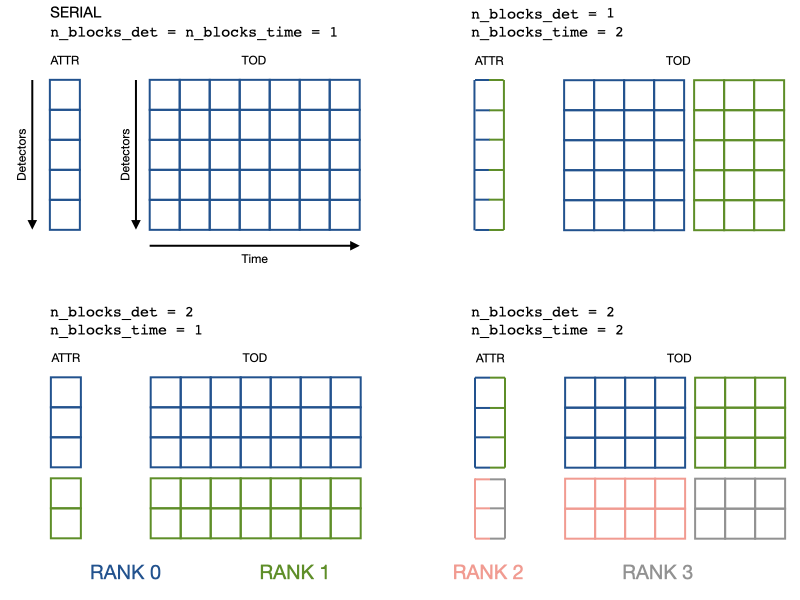
1. Uniform distribution of detectors along the detector axis#
With n_blocks_det and n_blocks_time arguments of Observation class,
the obs.tod is evenly distributed over a
n_blocks_det by n_blocks_time grid of MPI ranks. The blocks can be
changed at run-time.
The coherence between the serial and parallel operations is achieved by
distributing also the arrays of detector properties:
each rank keeps in memory only an interval of calibration_factors or
wn_levels, the same detector interval of tod.
The main advantage is that the example operations in the Serial section are achieved with the same lines of code. The price to pay is that you have to set detector properties with special methods.
import litebird_sim as lbs
from mpi4py import MPI

comm = MPI.COMM_WORLD

obs = lbs.Observation(
    detectors=2,
    start_time_global=0.0,
    sampling_rate_hz=5.0,
    n_samples_global=5,
    n_blocks_det=2, # Split the detector axis in 2
    comm=comm  # across the processes of this communicator
)

# Add detector properties either with a global array that contains
# all the detectors (which will be scattered across the processor grid)
obs.setattr_det_global('calibration_factors', np.array([1.1, 1.2]))

# Or with the local array, if somehow you have it already
if comm.rank == 0:
    wn_level_local = np.array([2.1])
elif comm.rank == 1:
    wn_level_local = np.array([2.2])
else:
    wn_level_local = np.array([])
obs.setattr_det('wn_levels', wn_level_local)

# Operate on the local portion of the data just like in serial code

# Apply to each detector its own calibration factor
obs.tod *=  obs.calibration_factors[:, None]

# Add white noise at a different level for each detector
obs.tod += (np.random.normal(size=obs.tod.shape)
            * obs.wn_levels[:, None])

# Change the data distribution
obs.set_blocks(n_blocks_det=1, n_blocks_time=1)
# Now the rank 0 has exactly the data of the serial obs object
For clarity, here is a visualization of how data (a detector attribute and the TOD) gets distributed.
2. Custom grouping of detectors along the detector axis#
While uniform distribution of detectors along the detector axis optimizes load
balancing, it is less suitable for simulating some effects, like crosstalk and
noise correlation between the detectors. For these effects, uniform distribution
across MPI processes necessitates the transfer of large TOD arrays across multiple
MPI processes, which complicates the code implementation and may potentially lead
to significant performance overhead. To save us from this situation, the
Observation class
accepts an argument det_blocks_attributes that is a list of string objects
specifying the detector attributes to create the group of detectors. Once the
detector groups are made, the detectors are distributed to the MPI processes in such
a way that all the detectors of a group reside on the same set of MPI processes.
If a valid det_blocks_attributes argument is passed to the Observation
class, the arguments n_blocks_det and n_blocks_time are ignored. Since the
det_blocks_attributes creates the detector blocks dynamically, the
n_blocks_time is computed during runtime using the size of MPI communicator and
the number of detector blocks (n_blocks_time = comm.size // n_blocks_det).
The detector blocks made in this way can be accessed with
Observation.detector_blocks. It is a dictionary object that has the tuple of
det_blocks_attributes values as dictionary keys and the list of detectors
corresponding to the key as dictionary values. This dictionary is sorted so that the
group with the largest number of detectors comes first and the one with
the fewest detectors comes last.
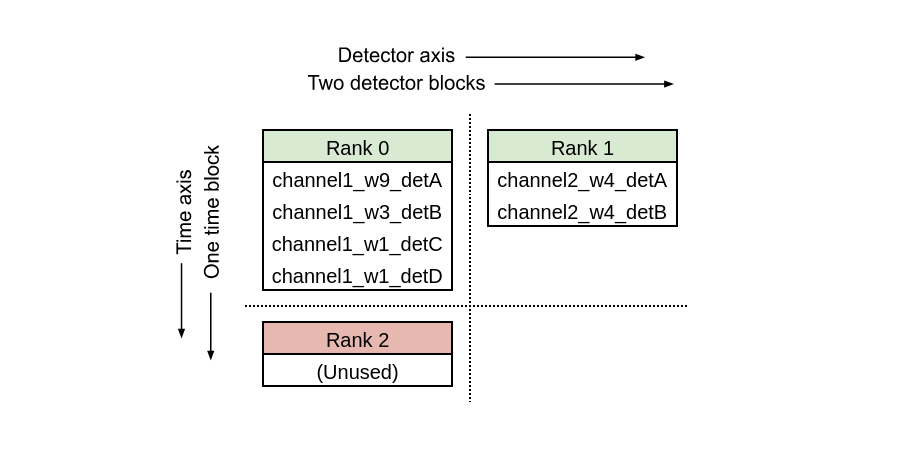
The following example illustrates the distribution of obs.tod matrix across the
MPI processes when det_blocks_attributes is specified.
import litebird_sim as lbs

comm = lbs.MPI_COMM_WORLD

start_time = 456
duration_s = 100
sampling_freq_Hz = 1

# Creating a list of detectors.
dets = [
    lbs.DetectorInfo(
        name="channel1_w9_detA",
        wafer="wafer_9",
        channel="channel1",
        sampling_rate_hz=sampling_freq_Hz,
    ),
    lbs.DetectorInfo(
        name="channel1_w3_detB",
        wafer="wafer_3",
        channel="channel1",
        sampling_rate_hz=sampling_freq_Hz,
    ),
    lbs.DetectorInfo(
        name="channel1_w1_detC",
        wafer="wafer_1",
        channel="channel1",
        sampling_rate_hz=sampling_freq_Hz,
    ),
    lbs.DetectorInfo(
        name="channel1_w1_detD",
        wafer="wafer_1",
        channel="channel1",
        sampling_rate_hz=sampling_freq_Hz,
    ),
    lbs.DetectorInfo(
        name="channel2_w4_detA",
        wafer="wafer_4",
        channel="channel2",
        sampling_rate_hz=sampling_freq_Hz,
    ),
    lbs.DetectorInfo(
        name="channel2_w4_detB",
        wafer="wafer_4",
        channel="channel2",
        sampling_rate_hz=sampling_freq_Hz,
    ),
]

# Initializing a simulation
sim = lbs.Simulation(
    start_time=start_time,
    duration_s=duration_s,
    random_seed=12345,
    mpi_comm=comm,
)

# Creating the observations with detector blocks
sim.create_observations(
    detectors=dets,
    split_list_over_processes=False,
    num_of_obs_per_detector=3,
    det_blocks_attributes=["channel"], # case 1 and 2
    # det_blocks_attributes=["channel", "wafer"] # case 3
)
With the list of detectors defined in the code snippet above, we can see how the
detectors axis and time axis is divided depending on the size of MPI communicator and
det_blocks_attributes.
Case 1
Size of global MPI communicator = 3, det_blocks_attributes=["channel"]
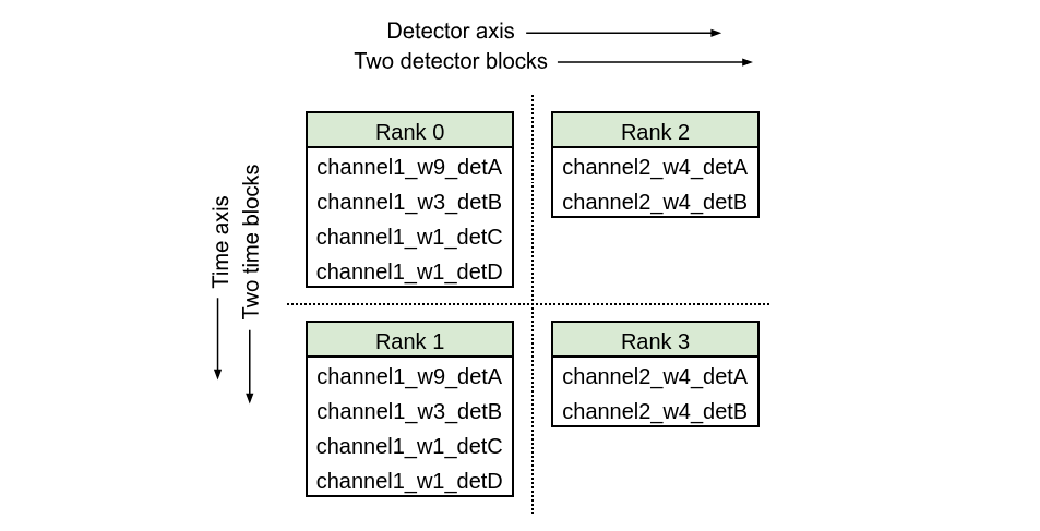
Case 2
Size of global MPI communicator = 4, det_blocks_attributes=["channel"]
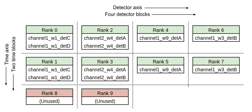
Case 3
Size of global MPI communicator = 10, det_blocks_attributes=["channel", "wafer"]
Note
When n_blocks_det != 1, keep in mind that obs.tod[0] or
obs.wn_levels[0] are quantities of the first local detector, not global.
This should not be a problem as the only thing that matters is that the two
quantities refer to the same detector. If you need the global detector index,
you can get it with obs.det_idx[0], which is created at construction time.
obs.det_idx stores the detector indices of the detectors available to an
Observation class, with respect to the list of detectors stored in
obs.detectors_global variable.
Note
To get a better understanding of how observations are being used in a
MPI simulation, use the method Simulation.describe_mpi_distribution().
This method must be called after the observations have been allocated using
Simulation.create_observations(); it will return an instance of the
class MpiDistributionDescr, which can be inspected to determine
which detectors and time spans are covered by each observation in all the
MPI processes that are being used. For more information, refer to the Section
Simulations.
MPI communicators#
The simulation framework exposes MPI communicators at different
levels. The first one is the global MPI communicator. It can be
accessed with a global variable MPI_COMM_WORLD, and it is
same as mpi4py.MPI.COMM_WORLD. It contains all the MPI processes
used by the script. The other MPI communicators defined in the
simulation framework are the partitions of global MPI communicator and
they contain the MPI processes that have certain properties as we
explain below. For all the examples in this sub-section, we consider
the distribution of TODs across 10 MPI processes with n_blocks_time = 2
and n_blocks_det = 4.
To distribute the TODs across
n_blocks_det \(\times\) n_blocks_time \(=\, N\)
MPI ranks, it is necessary that the script is executed with at least
\(N\) MPI processes. There is, however, no upper limit on the
number of MPI processes to be used. When the number of MPI processes
is higher than \(N\), it leaves all the MPI processes with
rank \(\geq N\) with no detector (and TOD). In many cases, it
is useful to identify the unused ranks so that they can be avoided
while performing some computations. The Observation class
makes this happen by making a sub-communicator containing only the
processes that contain a non-zero number of detectors (and TODs).
However, once the detectors and TODs are distributed across several
processes, it is not trivial to find out all the ranks that contain
the TOD chunks of a given detector (or detector block). Likewise, it
is hard to find all the ranks that contain the TOD chunks
corresponding to the same time interval. To solve this issue, Observation
class provides the MPI sub-communicators corresponding to different
groups of MPI processes.
The three sub-communicators provided by the framework - each generated by splitting the global MPI communicator - are listed below. The process ranks in the sub-communicators are based on the order of their global ranks:
Grid communicator: Once the number of detector blocks and the number of time blocks are available, the Observation class splits the global communicator into a grid communicator and a null communicator. Grid communicator consist all the mpi processes whose rank is less than \(N\). The null communicator contains all other MPI processes. On the MPI processes with global rank less than \(N\), the global variable
MPI_COMM_GRID.COMM_OBS_GRIDpoints to the grid communicator. On other MPI processes, it points to the null MPI communicator (MPI_COMM_GRID.COMM_NULLwhich is same asmpi4py.MPI.COMM_NULL). In the example below, the processes with global rank from 0 to 7 belong to the grid sub-communicator. Since the processes with rank 8 and 9 are unused, they are excluded from the grid communicator.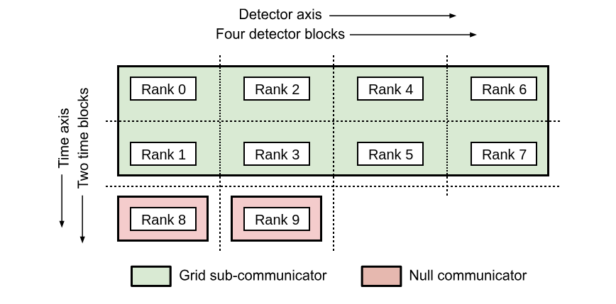
Note that, to exclude the MPI processes belonging to the null communicator from the computations, one should enclose the computations under an if condition comparing
MPI_COMM_GRID.COMM_OBS_GRIDagainstMPI_COMM_GRID.COMM_NULL:if MPI_COMM_GRID.COMM_OBS_GRID != MPI_COMM_GRID.COMM_NULL: # proceed with the following computations when # MPI_COMM_GRID.COMM_OBS_GRID is not null ...
Detector-block communicator: The detector-block communicator is made by splitting the grid communicator into
n_blocks_detsub-communicators, such that each sub-communicator contains the processes where TODs of the same set of detectors reside. This sub-communicator can be accessed withcomm_det_blocksattribute of theObservationclass. In the following example, the grid communicator is split into 4 detector-block communicators containing the processes with global rank 0-1, 2-3, 4-5, and 6-7 respectively.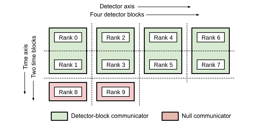
Time-block communicator: The time-block communicator is made by splitting the grid communicator into
n_blocks_timesub-communicators, such that each sub-communicator contains the processes where TOD chunks of same time interval reside. This sub-communicator can be accessed withcomm_time_blockattribute of theObservationclass. In the example below, the grid communicator is split into 2 time-block communicators containing the processes with global rank 0-2-4-6 and 1-3-5-7 respectively.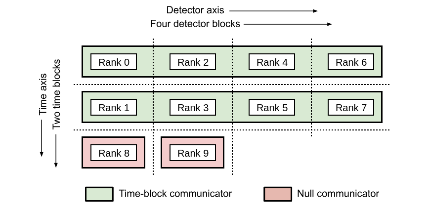
Other notable functionalities#
The starting time can be represented either as floating-point values (appropriate in 99% of the cases) or MJD; in the latter case, it is handled through the AstroPy library.
Instead of adding detector attributes after construction, you can pass a list of dictionaries (one entry for each detectors). One attribute is created for every key.
import litebird_sim as lbs
from astropy.time import Time

# Second case: use MJD to track the time
obs_mjd = lbs.Observation(
    detectors=[{"name": "A"}, {"name": "B"}],
    start_time_global=Time("2020-02-20", format="iso"),
    sampling_rate_hz=5.0,
    n_samples_global=5,
)

obs.name == np.array(["A", "B"])  # True
Obtain pointings#
The pointing information for one or more detectors in an observation are
accessible through the get_pointings() which returns a tuple containing
the pointing matrix of the detectors and the HWP angle. This call must be prepared
calling either the method Observation.prepare_pointings() of this class or
Simulation.prepare_pointings(), or the function litebird_sim.prepare_pointings()
The structure of the pointing matrix returned depends on the parameter detector_idx that specifies which detectors should be included in the computation. The following calls are all legitimate.
# All the detectors are included
pointings, hwp_angle = cur_obs.get_pointings("all")
# This returns ``(N_det, N_samples, 3)`` array

# Only the first two detectors are included
pointings, hwp_angle = cur_obs.get_pointings([0, 1])
# This returns ``(2, N_samples, 3)`` array

# Only the first detector is used
pointings, hwp_angle = cur_obs.get_pointings(0)
# This returns ``(N_samples, 3)`` array

# NB if a list of indices is passed an array of dimension ``(N_det, N_samples, 3)``
# is always returned
# For example this
pointings, hwp_angle = cur_obs.get_pointings([0])
# returns ``(1, N_samples, 3)`` array
The last dimension spans the three angles θ (colatitude, in radians), φ (longitude, in
radians), and ψ (orientation angle, in radians).
The HWP angle is always a vector with shape (N_samples,), as it does not depend on
the list of detectors.
The method get_hwp_angle() allows to obtain only the HWP angle.
The function litebird_sim.precompute_pointings() precomputes all the pointings
for a set of observations storing them in Observation.pointing_matrix and
Observation.hwp_angle. See above for more details. The same result is achieved
calling the method Observation.precompute_pointings().
Reading/writing observations to disk#
The framework implements a couple of functions to write/read
Observation objects to disk, using the HDF5 file format. By
default, each observation is saved in a separate HDF5 file; the
following information are saved and restored:
Whether times are tracked as floating-point numbers or proper AstroPy dates;
The TOD matrix (in
.tod);The quaternions used to create the pointings.
Optionally, full pointings can be computed on the fly and stored in the files; this is useful if the TOD is supposed to be read by some other program.
Global and local flags saved in
.global_flagsand.local_flags(see below).
The function used to save observations is Simulation.write_observations(),
which acts on a Simulation object; if you prefer to
operate without a Simulation object, you can call
write_list_of_observations().
To read observations, you can use Simulation.read_observations() and
read_list_of_observations().
The framework writes one HDF5 file for each Observation; each
file contains the following datasets:
One dataset per each TOD; each dataset has the same name as the ones passed to
tods=in the call tocreate_observations. It has the following attributes:use_mjd(Boolean):Trueifstart_timeis a MJD,Falseif it is a plain floating-point valuestart_time(Float): the time of the first sample in the TOD, see alsouse_mjdto correctly interpret thissampling_rate_hz(Float)detectors(string): a JSON record containing basic information about the detectorsdescription(string): a human-readable string describing what’s in this TOD
global_flags: the matrix of the global flags for the observationflags_NNNN`: the local flags for detector ``NNNN(starting from0000). There are as many datasets of this kind as the number of detectors in thisObservationobject.pointing_provider_rot_quaternion: the rotation quaternion that converts the boresight direction of the focal plane of the instrument into ecliptic coordinates. It is a matrix with shape(N, 4), and it has the attributesstart_time(either a floating-point value or a string, the latter being used forastropy.time.Timetypes) andsampling_rate_hz.pointing_provider_hwp: a dataset containing the details of the Half-Wave Plate. Its interprentation depends on the kind of HWP; for instances of the classIdealHWP, the dataset is empty and the only fields are the attributesclass_name(always equal toIdealHWP),ang_speed_radpsec, andstart_angle_rad(two floating-point numbers).rot_quaternion_NNNN: the rotation quaternion for detectorNNNN(starting from0000). It has the same structure aspointing_provider_rot_quaternion(see above), and there are as many datasets of this kind as the number of detectors in thisObservationobject.
Flags#
The LiteBIRD Simulation Framework permits to associate flags with the scientific samples in a TOD. These flags are usually unsigned integer numbers that are treated like bitmasks that signal peculiarities in the data. They are especially useful when dealing with data that have been acquired by some real instrument to signal if the hardware was malfunctioning or if some disturbance was recorded by the detectors. Other possible applications are possible:
Marking samples that should be left out of map-making (e.g., because a planet or some other transient source was being observed by the detector).
Flagging potentially interesting observations that should be used in data analysis (e.g., observations of the Crab nebula that are considered good enough for polarization angle calibration).
Similarly to other frameworks like TOAST, the LiteBIRD Simulation
Framework lets to store both «global» and «local» flags associated
with the scientific samples in TODs. Global flags are associated with
all the samples in an Observation, and they must be a vector of M
elements, where M is the number of samples in the TOD. Local
samples are stored in a matrix of shape N × M, where N is the
number of detectors in the observation.
The framework encourages to store these flags in the fields
local_flags and global_flags: in this way, they can be saved
correctly in HDF5 files by functions like write_observations().
API reference#
- class litebird_sim.observations.Observation(detectors: int | list[dict], n_samples_global: int, start_time_global: float | Time, sampling_rate_hz: float, allocate_tod=True, tods=None, det_blocks_attributes: list[str] | None = None, n_blocks_det=1, n_blocks_time=1, comm=None, root=0)#
Bases:
objectAn observation made by one or multiple detectors over some time window
After construction at least the following attributes are available
start_time()n_samples()tod()2D array (n_detectors by n_samples) stacking the times streams of the detectors.
- A note for MPI-parallel application: unless specified, all the
variables are local. Should you need the global counterparts, 1) think twice, 2) append _global to the attribute name, like in the following:
start_time_global()end_time_global()n_detectors_global()~ n_detectors * n_blocks_detn_samples_global()~ n_samples * n_blocks_time
Following the same philosophy,
get_times()returns the time stamps of the local time interval- Parameters:
detectors (int or list[dict]) – Either the number of detectors or a list of dictionaries with one entry for each detector. The keys of the dictionaries become attributes of the observation. If a detector is missing a key it will be set to
nan. If an MPI communicator is passed tocomm,detectorsis relevant only on therootprocess.n_samples_global (int) – The total number of samples in this observation (global, before any MPI splitting in time).
start_time_global (float or astropy.time.Time) – Start time of the observation. It can either be an
astropy.time.Timeinstance or a floating-point number. In the latter case, it must be expressed in seconds.sampling_rate_hz (float) – Sampling frequency, in Hertz.
allocate_tod (bool, optional) – If
True(default), allocate the TOD arrays described bytods. IfFalse, the corresponding attributes are created but set toNone. This can be useful for workflows that only need pointing or metadata.tods (list[TodDescription] or None, optional) –
List of TOD descriptors defining which TOD arrays should be attached to the observation. Each
TodDescriptionspecifies:name: attribute name of the 2D array;units: physical units as aUnitsitem (e.g.Units.K_CMB);dtype: NumPy dtype (e.g.numpy.float32);description: human-readable description.
If
None, a single TOD named"tod"with unitsUnits.K_CMBand dtypenumpy.float32is created.det_blocks_attributes (list[str] or None, optional) – List of detector attributes used to divide the detector axis of the TOD (and all detector-attribute arrays). For example, with
det_blocks_attributes = ["wafer", "pixel"], detectors are divided into blocks such that all detectors in a block share the samewaferandpixelattribute.n_blocks_det (int, optional) – Number of blocks used to divide the detector axis of the TOD (and the arrays of detector attributes). Ignored if
det_blocks_attributesis notNone.n_blocks_time (int, optional) – Number of blocks used to divide the time axis of the TOD. Ignored if
det_blocks_attributesis notNone.comm (MPI communicator or None, optional) – Either
None(do not use MPI) or an MPI communicator object, such asmpi4py.MPI.COMM_WORLD. Its size is required to be at leastn_blocks_det * n_blocks_time.root (int, optional) – Rank of the process receiving the detector list when
detectorsis a list of dictionaries; otherwise ignored.
- blms: dict | None#
- destriper_pixel_idx: ndarray[tuple[Any, ...], dtype[_ScalarT]] | None#
- destriper_pol_angle_rad: ndarray[tuple[Any, ...], dtype[_ScalarT]] | None#
- destriper_weights: ndarray[tuple[Any, ...], dtype[_ScalarT]] | None#
- det_idx: ndarray[tuple[Any, ...], dtype[_ScalarT]]#
- ellipticity: ndarray[tuple[Any, ...], dtype[_ScalarT]]#
- fwhm_arcmin: ndarray[tuple[Any, ...], dtype[_ScalarT]]#
- get_delta_time() float | TimeDelta#
Return the time interval between two consecutive samples in this observation
Depending whether the field
start_timeof theObservationobject is afloator aastropy.time.Timeobject, the return value is either afloat(in seconds) or an instance ofastropy.time.TimeDelta. See alsoget_time_span().
- get_hwp_angle(hwp_buffer: ~numpy.ndarray[tuple[~typing.Any, ...], ~numpy.dtype[~numpy._typing._array_like._ScalarT]] | None = None, pointings_dtype=<class 'numpy.float64'>) ndarray[tuple[Any, ...], dtype[_ScalarT]] | None#
Compute the Half-Wave Plate (HWP) angle for this observation.
This method triggers the time-domain computation of the HWP angle using the internally stored
PointingProvider. It returns a NumPy array of shape (n_samples,) containing the HWP angle in radians for the entire duration of the observation.If the observation does not include a Half-Wave Plate, the method returns None.
- Parameters:
hwp_buffer (np.ndarray, optional) – Optional pre-allocated array of shape (n_samples,) in which to store the HWP angle values. If not provided, a new buffer will be allocated.
pointings_dtype (data-type, optional) – Data type to use when allocating the HWP buffer, if needed. Defaults to np.float64.
- Returns:
The array containing the computed HWP angles (in radians), or None if no HWP is configured for the observation.
- Return type:
np.ndarray or None
- Raises:
AssertionError – If the pointing_provider has not been initialized (e.g., prepare_pointings() has not been called), or if the provided hwp_buffer does not match the expected shape.
Example
hwp_angle = obs.get_hwp_angle() hwp_angle.shape -> (obs.n_samples,)
- get_pointings(detector_idx: int | list[int] | str = 'all', pointing_buffer: ~numpy.ndarray[tuple[~typing.Any, ...], ~numpy.dtype[~numpy._typing._array_like._ScalarT]] | None = None, hwp_buffer: ~numpy.ndarray[tuple[~typing.Any, ...], ~numpy.dtype[~numpy._typing._array_like._ScalarT]] | None = None, pointings_dtype=<class 'numpy.float64'>, nside_centering: int | None = None, nthreads: int | None = None) tuple[ndarray[tuple[Any, ...], dtype[_ScalarT]], ndarray[tuple[Any, ...], dtype[_ScalarT]] | None]#
Compute the pointings for one or more detectors in this observation
This method triggers the computation of the matrix of pointings that indicate the direction of the line of sight for each sample in the TOD of the current
Observationinstance. You must call eitherprepare_pointings()orSimulation.prepare_pointings()before invoking this method.The parameter detector_idx specifies which detectors should be included in the computation. Use
"all"to ask for the pointings of all the detectors in this Observation; if you just want a subset of them, pass a list with their zero-based index; if you just want the pointings for one detector, you can pass an integer. The following calls are all legitimate:# All the detectors are included pointings, hwp_angle = cur_obs.get_pointings("all") # This returns ``(N_det, N_samples, 3)`` array # Only the first two detectors are included pointings, hwp_angle = cur_obs.get_pointings([0, 1]) # This returns ``(2, N_samples, 3)`` array # Only the first detector is used pointings, hwp_angle = cur_obs.get_pointings(0) # This returns ``(N_samples, 3)`` array # NB if a list of indices is passed an array of dimension ``(N_det, N_samples, 3)`` # is always returned # For example this pointings, hwp_angle = cur_obs.get_pointings([0]) # returns ``(1, N_samples, 3)`` array
The return value is a pair containing (1) the pointing matrix and (2) the HWP angle. The pointing matrix is a NumPy array with shape
(N_det, N_samples, 3), whereN_det` is the number of detectors and ``N_samplesis the number of samples in the TOD (the fieldObservation.n_samples). The last dimension spans the three angles θ (colatitude, in radians), φ (longitude, in radians), and ψ (orientation angle, in radians). Important: if you ask for just one detector passing the index of the detector, the shape of the pointing matrix will always be(N_samples, 3). The pointings can be aligned to the center of the HEALPix pixel setting nside_centering to the nside of an HEALPix map. The HWP angle is always a vector with shape(N_samples,), as it does not depend on the list of detectors.The return value is allocated internally by the method. If you instead want to pass a pre-allocated structure, you can use the pointing_buffer and hwp_buffer parameters. In this case, the return value will be always equal to
(pointing_buffer, hwp_buffer).
- get_time_span() float | TimeDelta#
Return the temporal length of the current observation
This method can either return a
float(in seconds) or aastropy.time.TimeDeltaobject, depending whether the fieldstart_timeof theObservationobject is afloator aastropy.time.Timeinstance. See alsoget_delta_time().
- get_times(normalize=False, astropy_times=False)#
Return a vector containing the time of each sample in the observation
The measure unit of the result depends on the value of astropy_times: if it’s true, times are returned as astropy.time.Time objects, which can be converted to several units (MJD, seconds, etc.); if astropy_times is false (the default), times are expressed in seconds. In the latter case, you should interpret these times as sidereal.
If normalize=True, then the first time is zero. Setting this flag requires that astropy_times=False.
This can be a costly operation; you should cache this result if you plan to use it in your code, instead of calling this method over and over again.
Note for MPI-parallel codes: the times returned are only those of the local portion of the data. This means that
the size of the returned array is
n_samples, smaller thann_samples_globalwhenever there is more than one time-blockself.tod * self.get_times()is a meaningless but always allowed operation
- jones_hwp: list#
- local_flags: ndarray[tuple[Any, ...], dtype[_ScalarT]] | None#
- mueller_hwp: ndarray[tuple[Any, ...], dtype[_ScalarT]]#
- property n_blocks_det#
- property n_blocks_time#
- property n_detectors#
- property n_detectors_global#
Total number of detectors in the observation
If you need the number of detectors in the local TOD block
self.tod, use eithern_detectorsorself.tod.shape[0].
- property n_samples_global#
Samples in the whole observation
If you need the time-lenght of the local TOD block
self.tod, use eithern_samplesorself.tod.shape[1].
- name: list#
- net_ukrts: int | float | ndarray[tuple[Any, ...], dtype[_ScalarT]]#
- pol_angle_rad: ndarray[tuple[Any, ...], dtype[_ScalarT]]#
- precompute_pointings(pointings_dtype=<class 'numpy.float64'>) None#
Precompute and store the full pointing matrix and HWP angles for this observation.
This method computes the time-domain pointing angles (θ, φ, ψ) and, if applicable, HWP angles for all detectors in the current observation. The results are stored in the fields self.pointing_matrix and self.hwp_angle.
This is typically used to cache the pointings when running in a mode that avoids on-the-fly computation.
- Parameters:
pointings_dtype (data-type, optional) – Data type to use for the computed arrays. Defaults to np.float64.
- Raises:
AssertionError – If prepare_pointings() has not been called prior to this method, i.e., if self.pointing_provider is not defined.
Notes
This method must be called after prepare_pointings().
- prepare_pointings(instrument: InstrumentInfo, spin2ecliptic_quats: RotQuaternion, hwp: HWP | None = None, maximum_internal_buffer_mem_mb: float = 256.0) None#
Prepare quaternion-based pointing and HWP information for this observation.
This method initializes the
PointingProviderused to compute time-dependent detector pointing angles (θ, φ, ψ) and, optionally, HWP angles. It combines the global spin-to-Ecliptic quaternions with the instrument’s internal boresight-to-spin rotation to produce a final boresight-to-Ecliptic quaternion, which is stored internally.If a Half-Wave Plate (HWP) model is provided, it is attached to the pointing provider and its Mueller matrix is applied to all detectors that do not already have one assigned. If no HWP is passed, all detectors must already define their own Mueller matrices.
- Parameters:
instrument (InstrumentInfo) – The instrument definition containing the boresight-to-spin rotation.
spin2ecliptic_quats (RotQuaternion) – Time-dependent rotation from the spin frame to the Ecliptic frame. Typically generated using
ScanningStrategy.generate_spin2ecl_quaternions().hwp (HWP | None) – Optional HWP model. If provided, it is stored and its Mueller matrix applied to all detectors lacking one.
maximum_internal_buffer_mem_mb (float) – Maximum number of megabytes (MB) to allocate for internal buffers during the computation of pointings. Set to -1 to remove any limit.
- Raises:
AssertionError – If hwp is not provided and one or more detectors do not have a pre-assigned Mueller matrix.
Notes
After calling this method, the observation becomes ready to compute pointings via
get_pointings()orget_hwp_angle()using its internalPointingProvider.
- psi_rad: ndarray[tuple[Any, ...], dtype[_ScalarT]]#
- quat: list#
- property sampling_rate_hz#
- set_hwp(hwp)#
- set_n_blocks(n_blocks_det=1, n_blocks_time=1)#
Change the number of blocks
- Parameters:
n_blocks_det (int) – new number of blocks in the detector direction
n_blocks_time (int) – new number of blocks in the time direction
- setattr_det(name, info)#
Add a piece of information about the detectors
Store
infoas the attributenameof the observation. The difference with respect toself.name = info, relevant only in MPI programs, areinfois assumed to contain a number of elements equal toself.tod.shape[0]and to have the same order (info[i]is a property ofself.tod[i])When changing
n_blocks_det,set_n_blocks()is aware ofnameand will redistributeinfoin such a way thatself.name[i]is a property ofself.tod[i]in the new block distribution
- Parameters:
name (str) – Name of the detector information
info (array) – Information to be stored in the attribute
name. The array must contain one entry for each local detector.
- setattr_det_global(name, info, root=0)#
Add a piece of information on the detectors
Variant of
setattr_det()to be used when the information comes from a single MPI rank (root). In particular,In the
rootprocess,infois required to haven_detectors_globalelements (notself.tod.shape[1]). For other processes info is irrelevantinfois scattered from therootrank to the relevant processes inself.commso thatself.namewill haveself.tod.shape[0]elements on all the processes andself.name[i]is a property ofself.tod[i]When changing
n_blocks_det,set_n_blocks()is aware ofnameand will redistributeinfoin such a way thatself.name[i]is a property ofself.tod[i]in the new block distribution
- Parameters:
name (str) – Name of the information
info (array) – Array containing
n_detectors_globalentries. Relevant only for thrrootprocessroot (int) – Rank of the root process
- sky: HealpixMap | SphericalHarmonics | dict[str, HealpixMap | SphericalHarmonics | SkyGenerationParams] | dict[str, dict[str, HealpixMap | SphericalHarmonics]] | None#
- tod: ndarray[tuple[Any, ...], dtype[_ScalarT]]#
- wafer: str | None#
- class litebird_sim.observations.TodDescription(name: str, units: Units, dtype: Any, description: str)#
Bases:
objectA compact descriptor for a Time-Ordered Data (TOD) field stored in an
Observationobject.This field is used to pass information about one TOD in a
Observationobject. It is mainly used by the methodSimulation.create_observation()to figure out how much memory allocate and how to organize it.The class contains three fields:
- Parameters:
name (str) – Name of the attribute created inside each
Observationinstance.units (Units) – Physical units of the TOD, expressed as an item of
Units.dtype (Any) – NumPy dtype used for allocating the underlying array, e.g., numpy.float32
description (str) – Human-readable description of the TOD field.
Notes
This class only describes the TOD. Actual memory allocation is performed by
Simulation.create_observations()based on the list of provided descriptors.- description: str#
- dtype: Any#
- name: str#
- class litebird_sim.io.DetectorJSONEncoder(*, skipkeys=False, ensure_ascii=True, check_circular=True, allow_nan=True, sort_keys=False, indent=None, separators=None, default=None)#
Bases:
JSONEncoder- default(o)#
Implement this method in a subclass such that it returns a serializable object for
o, or calls the base implementation (to raise aTypeError).For example, to support arbitrary iterators, you could implement default like this:
def default(self, o):
    try:
        iterable = iter(o)
    except TypeError:
        pass
    else:
        return list(iterable)
    # Let the base class default method raise the TypeError
    return super().default(o)
- litebird_sim.io.read_list_of_observations(file_name_list: list[str | ~pathlib.Path], tod_dtype=<class 'numpy.float32'>, limit_mpi_rank: bool = True, tod_fields: list[str | ~litebird_sim.observations.TodDescription] = ['tod']) list[Observation]#
Read a list of HDF5 files containing TODs and return a list of observations
The function reads all the HDF5 files listed in file_name_list (either a list of strings or
pathlib.Pathobjects) and assigns them to the various MPI processes that are currently running, provided that limit_mpi_rank isTrue; otherwise, all the files are read by the current process and returned in a list. By default, only thetodfield is loaded; if the HDF5 file contains multiple TODs, you must load each of them.When using MPI, the observations are distributed among the MPI processes using the same layout that was used to save them; this means that you are forced to use the same number of processes you used when saving the files. This number is saved in the attribute
mpi_sizein each of the HDF5 files.If the HDF5 file contains more than one TOD, e.g., foregrounds, dipole, noise…, you can specify which datasets to load with
tod_fields(a list of strings orTodDescriptionobjects). When passingTodDescriptioninstances, only the name is used to select the dataset; dtype, units, and description are taken from the HDF5 attributes when present. Each dataset is initialized as a member field of theObservationclass, likeObservation.tod.
- litebird_sim.io.read_one_observation(path: str | ~pathlib.Path, limit_mpi_rank=True, tod_dtype=<class 'numpy.float32'>, read_quaternions_if_present=True, read_global_flags_if_present=True, read_local_flags_if_present=True, tod_fields: list[str] = ['tod']) Observation | None#
Read one
Observationobject from a HDF5 file.This is a low-level function that is wrapped by
read_list_of_observations()andread_observations(). It returns aObservationobject filled with the data read from the HDF5 file pointed by path.If limit_mpi_rank is
True(the default), the function makes sure that the rank of the MPI process reading this file is the same as the rank of the process that originally wrote it.The flags tod_dtype permits to override the data type of TOD samples used in the HDF5 file.
The parameters read_global_flags_if_present, and read_local_flags_if_present permit to avoid loading some parts of the HDF5 if they are not needed.
The parameter tod_fields specifies which TOD datasets to load. It can be a list of strings (dataset names) or
TodDescriptionobjects; in the latter case, only the name is used to find the dataset, while dtype, units, and description are read from the file when present.The function returns a
Observation, orNothingif the HDF5 file was ill-formed.
- litebird_sim.io.read_pointing_provider_from_hdf5(input_file: File, field_name: str) PointingProvider#
- litebird_sim.io.read_rot_quaternion_from_hdf5(input_file: File, field_name: str) RotQuaternion#
- litebird_sim.io.write_list_of_observations(observations: ~litebird_sim.observations.Observation | list[~litebird_sim.observations.Observation], path: str | ~pathlib.Path, tod_dtype=<class 'numpy.float32'>, pointings_dtype=<class 'numpy.float64'>, file_name_mask: str = 'litebird_tod{global_index:04d}.h5', custom_placeholders: list[dict[str, ~typing.Any]] | None = None, start_index: int = 0, collective_mpi_call: bool = True, tod_fields: list[str | ~litebird_sim.observations.TodDescription] = [], gzip_compression: bool = False, write_full_pointings: bool = False) list[Path]#
Save a list of observations in a set of HDF5 files
This function takes one or more observations and saves the TODs in several HDF5 (each observation leads to one file), using tod_dtype and pointings_dtype as the default datatypes for the samples and the pointing angles. The function returns a list of the file written (
pathlib.Pathobjects).By default, this function only saves the TODs and the quaternions necessary to compute the pointings; if you want the full pointing information, i.e., the angles θ (colatitude), φ (longitude), ψ (orientation) and α (HWP angle), you must set write_full_pointings to
True.The name of the HDF5 files is built using the variable file_name_mask, which can contain placeholders in the form
{name}, wherenamecan be one of the following keys:mpi_rank: the rank number of the MPI process that owns this observation (starting from zero)mpi_size: the number of running MPI processesnum_of_obs: the number of observationsglobal_index: an unique increasing index identifying this observation among all the observations used by MPI processes (see below)local_index: the number of the current observation within the current MPI process (see below)
You can provide other placeholders through custom_placeholders, which must be a list of dictionaries. The number of elements in the list must be the same as the number of observations, and each dictionary will be used to determine the placeholders for the file name related to the corresponding observation. Here is an example:
custom_dicts = [
    { "myvalue": "A" },
    { "myvalue": "B" },
]

write_list_of_observations(
    observations=[obs1, obs2],  # Write two observations
    path=".",
    file_name_mask="tod_{myvalue}.h5",
    custom_placeholders=custom_dicts,
)

# The two observations will be saved in
# - tod_A.h5
# - tod_B.h5
If the parameter collective_mpi_call is
Trueand MPI is enabled (seelitebird_sim.MPI_ENABLED), the code assumes that this function was called at the same time by all the MPI processes that are currently running. This is the most typical case, i.e., you have several MPI processes and want that each of them save their observations in HDF5 files. Passcollective_mpi_call=Falseonly if you are calling this function on some of the MPI processes. Here is an example:if lbs.MPI_COMM_WORLD.rank == 0: # Do this only for the first MPI process write_list_of_observations( ..., collective_mpi_call=False, )
In the example,
collective_mpi_call=Falsesignals that not every MPI process is writing their observations to disk.The
local_indexandglobal_indexplaceholders used in the template file name start from zero, but this can be changed using the parameter start_index.If observations contain more than one timeline in separate fields (e.g., foregrounds, dipole, noise…), you can specify the names of the fields using the parameter
tod_fields(list of strings orTodDescriptionobjects), which by default will only save Observation.tod.To save disk space, you can choose to apply GZip compression to the data frames in each HDF5 file (the file will still be a valid .h5 file).
- litebird_sim.io.write_one_observation(output_file: File, obs: Observation, tod_dtype, pointings_dtype, global_index: int, local_index: int, tod_fields: list[str | TodDescription] | None = None, gzip_compression: bool = False, write_full_pointings: bool = False)#
Write one
Observationobject in a HDF5 file.This is a low-level function that stores a TOD in a HDF5 file. You should usually use more high-level functions that are able to write several observations at once, like
write_list_of_observations()andwrite_observations().By default, this function only saves the TODs and the quaternions necessary to compute the pointings; if you want the full pointing information, i.e., the angles θ (colatitude), φ (longitude), ψ (orientation) and α (HWP angle), you must set write_full_pointings to
True.The output file is specified by output_file and should be opened for writing; the observation to be written is passed through the observations parameter. The data type to use for writing TODs and pointings is specified in the tod_dtype and pointings_dtype (it can either be a NumPy type like
numpy.float64or a string, passNoneto use the same type as the one used in the observation). Note that quaternions are always saved using 64-bit floating point numbers.The global_index and local_index parameters are two integers that are used by high-level functions like
write_observations()to understand how to read several HDF5 files at once; if you do not need them, you can pass 0 to both.
- litebird_sim.io.write_pointing_provider_to_hdf5(output_file: File, field_name: str, pointing_provider: PointingProvider, compression: str | None)#
- litebird_sim.io.write_rot_quaternion_to_hdf5(output_file: File, rot_matrix: RotQuaternion, field_name: str, compression: str | None) Dataset#