Simulations#

The LiteBIRD Simulation Framework is built on the Simulation class, which should be instantiated in any pipeline built using this framework. The class acts as a container for the many analysis modules available to the user, and it offers the following features:

Provenance model;
Interface with the instrument database;
System abstractions;
High level interface for simulation modules;
Generation of reports;
Printing status messages on the terminal (logging).

Provenance model #

A «provenance model» is, generally speaking, a way to track the history and origin of a data set by recording the following information:

Who or what created the dataset?
Which algorithm or instrumentation was used to produce it?
Which steps were undertaken to process the raw data?
How can one get access to the raw samples used to produce the dataset?

The LiteBIRD Simulation Framework tracks these information using parameter files (in TOML format), accessing the LiteBIRD Instrument Model (IMO) through the unique identifiers provided by the Data Access Layer (DAL), and generating reports after the simulation completes. Here is an example:

[general]
start_time = "2030-01-01T00:00:00"
duration_s = "720 days"

[detectors]
det_list = [
    "/releases/vPTEP/satellite/LFT/L1-040/000_000_003_QA_040_T/detector_info",
]

This text file can be provided as input to a Simulation object, which will use the information to set up the simulation.

Parameter files #

When you run a simulation, there are typically plenty of parameters that need to be passed to the code: the resolution of an output map, the names of the detectors to simulate, whether to include synchrotron emission in the sky model, etc.

The Simulation class eases this task by accepting the path to a TOML file as a parameter (parameter_file). Specifying this parameter triggers two actions:

The file is copied to the output directory where the simulation output files are going to be written (i.e., the same that contains report.html);
The file is read and made available in the field Simulation.parameters (a Python dictionary).

Using a parameter file is optional; if you do not specify parameter_file while creating a Simulation object, the parameters field will be set to an empty dictionary. (You can even directly pass a dictionary to a Simulation object: this can be handy if you already constructed a parameter object somewhere else.)

Take this example of a simple TOML file:

# This is file "my_conf.toml"
[simulation]
random_seed = 12345

[general]
nside = 512
imo_version = "v1.3"

[sky_model]
components = ["synchrotron", "dust", "cmb"]

The following example loads the TOML file and prints its contents to the terminal:

import litebird_sim as lbs

sim = lbs.Simulation(parameter_file="my_conf.toml")

print("Seed for the random number generator:",
      sim.parameters["simulation"]["random_seed"])
print("NSIDE =", sim.parameters["general"]["nside"])
print("The IMO I'm going to use is",
      sim.parameters["general"]["imo_version"])

print("Here are the sky components I'm going to simulate:")
for component in sim.parameters["sky_model"]["components"]:
    print("-", component)

The output of the script is the following:

Seed for the random number generator: 12345
NSIDE = 512
The IMO I'm going to use is v1.3
Here are the sky components I'm going to simulate:
- synchrotron
- dust
- cmb

A Simulation object only interprets the section simulation and leaves everything else unevaluated: it’s up to the simulation modules to make sense of any other section. The recognized parameters in the section named simulation are the following:

base_path: a string containing the path where to save the results of the simulation.
start_time: the start time of the simulation. If it is a string or a TOML datetime, it will be passed to the constructor for astropy.time.Time, otherwise it must be a floating-point value.
duration_s: a floating-point number specifying how many seconds the simulation should last. You can pass a string, which can contain a measurement unit as well: in this case, you are not forced to specify the duration in seconds. Valid units are: days (or day), hours (or hour), min, and sec (or s).
name: a string containing the name of the simulation.
description: a string containing a (possibly long) description of what the simulation does.
random_seed: the seed for the random number generator. An integer value ensures the reproducibility of the results obtained with random numbers; by passing None there will not be the possibility to re-obtain the same outputs. You can find more details in Random numbers.
numba_num_of_threads: number of threads used by Numba when running a parallel calculation.
numba_threading_layer: the multi-threading library to be used by Numba for parallel computations. See the Numba user’s manual to check which choices are available.

These parameters can be used instead of the keywords in the constructor of the Simulation class. Consider the following code:

sim = lbs.Simulation(
    base_path="/storage/output",
    start_time=astropy.time.Time("2020-02-01T10:30:00"),
    duration_s=3600.0,
    name="My simulation",
    description="A long description should be put here",
    random_seed=12345,
    numba_num_of_threads=4,
    numba_threading_layer="workqueue",
)

You can achieve the same if you create a TOML file named foo.toml that contains the following lines:

[simulation]
base_path = "/storage/output"
start_time = 2020-02-01T10:30:00
duration_s = 3600.0
name = "My simulation"
description = "A long description should be put here"
random_seed = 12345
numba_num_of_threads = 4
numba_threading_layer = "workqueue"

and then you initialize the sim variable in your Python code as follows:

sim = lbs.Simulation(parameter_file="foo.toml")

A nice feature of the framework is that the duration of the mission must not be specified in seconds. You would achieve identical results if you specify the duration in one of the following ways:

# All of these are the same
duration_s = "1 hour"
duration_s = "60 min"
duration_s = "3600 s"

Interface with the instrument database #

To simulation LiteBIRD’s data acquisition, the simulation code must be aware of the characteristics of the instrument. These are specified in the LiteBIRD Instrument Model (IMO) database, which can be accessed by people with sufficient rights. This Simulation Framework has the ability to access the database and take the input parameters necessary for its analysis modules to produce the expected output.

System abstractions #

In some cases, simulations must be ran on HPC computers, distributing the job on many processing units; in other cases, a simple laptop might be enough. The LiteBIRD Simulation Framework uses MPI to parallelize its codes, which is however an optional dependency: the code can be ran serially.

If you want to use MPI in your scripts, assuming that you have created a virtual environment as explained in the Tutorial, you have just to install mpi4py:

# With uv (recommended)
$ uv sync --extra mpi

# With pip
$ pip install mpi4py

# Always do this after "pip install", it will record the
# version number of mpi4py and all the other libraries
# you have installed in your virtual environment
$ pip freeze > requirements.txt

# Run the program using 4 processes
$ mpiexec -n 4 python3 my_script.py

The framework will detect the presence of mpi4py, and it will automatically use distributed algorithms where applicable; otherwise, serial algorithms will be used. You can configure this while creating a Simulation object:

import litebird_sim as lbs
import mpi4py

# This simulation *must* be ran using MPI
sim = lbs.Simulation(mpi_comm=mpi4py.MPI.COMM_WORLD, random_seed=12345)

The framework sets a number of variables related to MPI; these variables are always defined, even if MPI is not available, and they can be used to make the code work in serial environments too. If your code must be able to run both with and without MPI, you should initialize a Simulation object using the variable MPI_COMM_WORLD, which is either mpi4py.MPI.COMM_WORLD (the default MPI communicator) or a dummy class if MPI is disabled:

import litebird_sim as lbs

# This simulation can take advantage of MPI if present,
# otherwise it will stick to serial execution
sim = lbs.Simulation(mpi_comm=lbs.MPI_COMM_WORLD, random_seed=12345)

See the page Multithreading and MPI for more information.

Generation of reports #

This section should explain how reports can be generated, first from the perspective of a library user, and then describing how developers can generate plots for their own modules.

Here is an example, showing several advanced topics like mathematical formulae, plots, and value substitution:

import litebird_sim as lbs
import matplotlib.pylab as plt

sim = lbs.Simulation(
    name="My simulation",
    base_path="output",
    random_seed=12345,
)
data_points = [0, 1, 2, 3]

plt.plot(data_points)
fig = plt.gcf()

sim.append_to_report('''
Here is a formula for $`f(x)`$:

```math
f(x) = \sin x
```

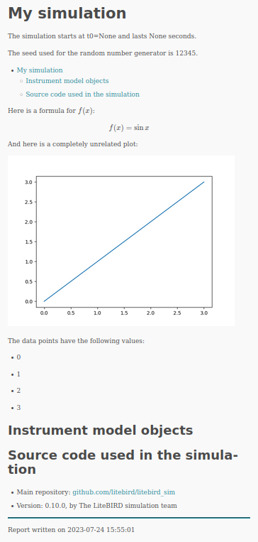
And here is a completely unrelated plot:

![](myplot.png)

The data points have the following values:
{% for sample in data_points %}
- {{ sample }}
{% endfor %}
''', figures=[(fig, "myplot.png")],
     data_points=data_points)

sim.flush()

And here is the output, which is saved in output/report.html:

Logging #

The report generation tools described above are useful to produce a synthetic report of the scientific outcomes of a simulation. However, one often wants to monitor the execution of the code in a more detailed manner, checking which functions have been called, how often, etc. In this case, the best option is to write messages to the terminal. Python provides the logging module for this purpose, and when you initialize a Simulation object, the module is initialized with a set of sensible defaults. In your code you can use the functions debug, info, warning, error, and critical to monitor what’s happening during execution:

import litebird_sim as lbs
import logging as log       # "log" is shorter to write
my_sim = lbs.Simulation(random_seed=12345)
log.info("the simulation starts here!")
pi = 3.15
if pi != 3.14:
    log.error("wrong value of pi!")

The output of the code above is the following:

[2020-07-18 06:25:27,653 INFO] the simulation starts here!
[2020-07-18 06:25:27,653 ERROR] wrong value of pi!

Note that the messages are prepended with the date, time, and level of severity of the message.

A few environment variables can taylor the way logging is done:

LOG_DEBUG: by default, debug messages are not printed to the terminal, because they are often too verbose for typical uses. If you want to debug your code, set a non-empty value to this variable.
LOG_ALL_MPI: by default, if you are using MPI then only messages from the process running with rank 0 will be printed. Setting this environment variable will make all the processes print their message to the terminal. (Caution: there might be overlapping messages, if two processes happen to write at the same time.)

The way you use these variable from the terminal is illustrated with an example. Suppose that we changed our example above, so that log.debug is called instead of log.info:

import litebird_sim as lbs
import logging as log  # "log" is shorter to write

my_sim = lbs.Simulation(random_seed=12345)
log.debug("the simulation starts here!")
pi = 3.15
if pi != 3.14:
    log.debug("wrong value of pi!")

In this case, running the script will produce no messages, as the default is to skip log.debug calls:

$ python my_script.py
$

However, running the script with the environment variable LOG_DEBUG set will make the messages appear:

$ LOG_DEBUG=1 python my_script.py
[2020-07-18 06:31:03,223 DEBUG] the simulation starts here!
[2020-07-18 06:31:03,224 DEBUG] wrong value of pi!
$

Monitoring MPI processes #

When using MPI, the method Simulation.create_observations() distributes detectors and time spans over all the available MPI processes, using the container object Observation to keep detectors, times, and pointing information in the same place. (See Observations for more information.) The Simulation class provides a method that enables the user to inspect how the TOD has been split among the many MPI processes: Simulation.describe_mpi_distribution().

The method must be called at the same time on all the MPI processess, once you have successfully called Simulation.create_observations():

import litebird_sim as lbs

# Be sure to create a `Simulation` object and create
# the observations:
#
#     sim = lbs.Simulation(…)
#     sim.create_observations(…)

# Now ask the framework to report how it's using each MPI process
descr = sim.describe_mpi_distribution()

The return type for Simulation.describe_mpi_distribution() is MpiDistributionDescr, which can be printed on the spot using print(descr). The result looks like the following example:

# MPI rank #1

## Observation #0
- Start time: 0.0
- Duration: 21600.0 s
- 1 detector(s) (0A)
- TOD(s): tod
- TOD shape: 1×216000
- Types of the TODs: float64

## Observation #1
- Start time: 43200.0
- Duration: 21600.0 s
- 1 detector(s) (0A)
- TOD(s): tod
- TOD shape: 1×216000
- Types of the TODs: float64

# MPI rank #2

## Observation #0
- Start time: 21600.0
- Duration: 21600.0 s
- 1 detector(s) (0A)
- TOD(s): tod
- TOD shape: 1×216000
- Types of the TODs: float64

## Observation #1
- Start time: 64800.0
- Duration: 21600.0 s
- 1 detector(s) (0A)
- TOD(s): tod
- TOD shape: 1×216000
- Types of the TODs: float64

# MPI rank #3

## Observation #0
- Start time: 0.0
- Duration: 21600.0 s
- 1 detector(s) (0B)
- TOD(s): tod
- TOD shape: 1×216000
- Types of the TODs: float64

## Observation #1
- Start time: 43200.0
- Duration: 21600.0 s
- 1 detector(s) (0B)
- TOD(s): tod
- TOD shape: 1×216000
- Types of the TODs: float64

# MPI rank #4

## Observation #0
- Start time: 21600.0
- Duration: 21600.0 s
- 1 detector(s) (0B)
- TOD(s): tod
- TOD shape: 1×216000
- Types of the TODs: float64

## Observation #1
- Start time: 64800.0
- Duration: 21600.0 s
- 1 detector(s) (0B)
- TOD(s): tod
- TOD shape: 1×216000
- Types of the TODs: float64

The class MpiDistributionDescr contains a list of MpiProcessDescr, which describe the «contents» of each MPI process. The most important field in each MpiProcessDescr instance is observations, which is a list of MpiObservationDescr objects: it contains the size of the TOD array, the names of the detectors, and other useful information. Refer to the documentation of each class to know what is inside.

High level interface #

The class Simulation has a powerful high level interface that allows to quickly generate a scanning strategy, allocate the observations, generate simulated timelines cointaing signal, noise and dipole, build maps, and save(read) the entire simulation object. The syntax is straightforward:

sim = lbs.Simulation(...)

sim.set_scanning_strategy(...)
sim.set_instrument(...)

sim.set_detectors(...)
sim.create_observations(...)
sim.prepare_pointings()

sim.compute_pos_and_vel()
sim.add_dipole()

sim.fill_tods(...)
sim.add_noise(...)

result = sim.make_destriped_map(nside=nside)
healpy.mollview(result.destriped_map)

sim.write_observations(...)
sim.read_observations(...)

Dedicated functions can also take care of the input generation and of the beam convolution:

sky_params = lbs.SkyGenerationParams(...)
alms = sim.get_sky(parameters=sky_params)

blms = sim.get_gauss_beam_alms(...)

Convparams = lbs.BeamConvolutionParameters(...)
sim.convolve_sky(sky_alms=alms,
                 beam_alms=blms,
                 convolution_params=Convparams,
                 ...,
                 )

TODs of the simulations can be also zeroed easly with:

sim.nullify_tod()

See the documentation in Observations, Scanning strategy Dipole anisotropy, Instrumental noise, Scanning a map to fill a TOD, Map-making, Convolve Alms with a Beam to fill a TOD, Synthetic Sky Maps, for details of the single functions.

The difference between the high-level and low-level interfaces is introduced in Interface Hierarchy and further explained in Appendix: why are there high- and low-level functions in LBS?.

Profiling a simulation #

The class Simulation provides an higher-level interface to the functions described in the chapter Profiling. The decorator @profile automatically wraps a method of the Simulation class so that it measures the time spent to run the method and adds it to an internal list of TimeProfiler objects. When the Simulation.flush() method is called, each MPI process creates its own JSON file containing the methods that have been measured during the execution of the simulation. These files are stored in the output directory and have names like profile_mpi00000.json, profile_mpi00001.json, etc.

Appendix: why are there high- and low-level functions in LBS?#

At the end of this chapter, it is useful to provide an explanation to the reason why Simulation provides methods that wrap functions, like Simulation.add_dipole() and add_dipole().

LBS is organized in a modular and hierarchical way because this facilitates flexibility and reuse. Functions like add_dipole() are meant to be used as low-level functions that perform the main computation. Often, there is a further split between the function that operates on one detector, like add_dipole_for_one_detector(), and the function that operates on many detectors at once, like add_dipole(); in this case, the former is usually implemented using Numba, while the latter is a plain for loop that wraps the former.

These low-level function usually require several parameters, but when they are called within large pipelines it is often the case that the same values would appear again and again as parameters to the many low-level functions needed in the simulation. For this reason, the constructor to Simulation asks for several parameters that are likely to be re-used, and it uses functions like Simulation.set_instrument() to inizialize member variables that are used by these high-level wrappers. In this way, the risk to mistakenly use two different values for the same parameter in the same simulation is minimized.

When implementing new modules, you should try to follow the same approach:

Implement a low-level function working on just one detector, if this is feasible for your purpose, and make it as efficient as possible. (Numba is a good choice here.)
Provide a function that iterates over many detectors and calls the function you just implemented. (Again, do this only if it makes sense.)
Implement a method in Simulation that wraps your function.

In a few cases, we choose to implement a new layer between point 2. and 3., where we wrap the low-level function in a method of the Observation class. In this case, the method in Simulation just iterates over Simulation.observations and calls it.

API reference #

class litebird_sim.simulations.MpiDistributionDescr(num_of_observations: int, detectors: list[DetectorInfo], mpi_processes: list[MpiProcessDescr])#

Bases: object

A class that describes how observations are distributed among MPI processes

The fields defined in this dataclass are the following:

num_of_observations (int): overall number of observations in all the MPI processes
detectors (list of DetectorInfo objects): list of all the detectors used in the observations
mpi_processes: list of MpiProcessDescr instances, describing the kind of data that each MPI process is currently holding

Use Simulation.describe_mpi_distribution() to get an instance of this object.

detectors: list[DetectorInfo]#

mpi_processes: list[MpiProcessDescr]#

num_of_observations: int#

class litebird_sim.simulations.MpiObservationDescr(det_names: list[str], tod_names: list[str], tod_shape: tuple[int, int] | None, tod_dtype: list[str], tod_description: list[str], start_time: float | Time, duration_s: float, num_of_samples: int, num_of_detectors: int)#

Bases: object

This class is used within MpiProcessDescr. It describes the kind and size of the data held by a Observation object.

Its fields are:

det_names (list of str): names of the detectors handled by this observation
tod_names (list of str): names of the fields containing the TODs (e.g., tod, cmb_tod, dipole_tod, …)
tod_shape (tuples of int): shape of each TOD held by the observation. This is not a list, because all the TODs are assumed to have the same shape
tod_dtype (list of str): string representing the NumPy data type of each TODs, in the same order as in the field tod_name
tod_description (list of str): list of human-readable descriptions for each TOD, in the same order as in the field tod_name
start_time (either a float or a astropy.time.Time): start date of the observation
duration_s (float): duration of the TOD in seconds
num_of_samples (int): number of samples held by this TOD
num_of_detectors (int): number of detectors held by this TOD. It’s the length of the field det_names (see above)

det_names: list[str]#

duration_s: float#

num_of_detectors: int#

num_of_samples: int#

start_time: float | Time#

tod_description: list[str]#

tod_dtype: list[str]#

tod_names: list[str]#

tod_shape: tuple[int, int] | None#

class litebird_sim.simulations.MpiProcessDescr(mpi_rank: int, numba_num_of_threads: int, observations: list[MpiObservationDescr])#

Bases: object

Description of the kind of data held by a MPI process

This class is used within MpiDistributionDescr. Its fields are:

mpi_rank: rank of the MPI process described by this instance
observations: list of MpiObservationDescr objects, each describing one observation managed by the MPI process with rank mpi_rank.
numba_num_of_threads (int): number of threads used by Numba
in the MPI process with rank mpi_rank.

mpi_rank: int#

numba_num_of_threads: int#

observations: list[MpiObservationDescr]#

class litebird_sim.simulations.OutputFileRecord(path, description)#

Bases: tuple

description#: Alias for field number 1

path#: Alias for field number 0

class litebird_sim.simulations.Simulation(random_seed='', base_path=None, name=None, mpi_comm=<litebird_sim.mpi._SerialMpiCommunicator object>, description='', start_time=None, duration_s=None, imo=None, parameter_file=None, parameters=None, numba_threads=None, numba_threading_layer=None, profile_time: bool = True)#

Bases: object

A container object for running simulations

This is the most important class in the Litebird_sim framework. It initializes an output directory that will contain all the products of a simulation and will handle the generation of reports and writing of output files.

Be sure to call Simulation.flush() when the simulation is completed. This ensures that all the information are saved to disk before the completion of your script.

You can access the fields base_path, name, mpi_comm, and description in the Simulation object:

sim = litebird_sim.Simulation(name="My simulation")
print(f"Running {sim.name}, saving results in {sim.base_path}")

The member variable observations is a list of Observation objects, which is initialized by the method create_observations().

This class keeps track of any output file saved in base_path through the member variable self.list_of_outputs. This is a list of objects of type OutputFileRecord(), which are 2-tuples of the form (path, description), where path is a pathlib.Path object and description is a str object:

for curpath, curdescr in sim.list_of_outputs:
    print(f"{curpath}: {curdescr}")

When pointing information is needed, you can call the method Simulation.set_scanning_strategy(), which initializes the members pointing_freq_hz and spin2ecliptic_quats; these members are used by functions like get_pointings().

Parameters:

random_seed (int or None) – the seed used for the random number generator. The user is required to set this parameter. By setting it to None, the generation of random numbers will not be reproducible.
base_path (str or pathlib.Path) – the folder that will contain the output. If this folder does not exist and the user has sufficient rights, it will be created.
name (str) – a string identifying the simulation. This will be used in the reports.
mpi_comm – either None (do not use MPI) or a MPI communicator object, like mpi4py.MPI.COMM_WORLD.
description (str) – a (possibly long) description of the simulation, to be put in the report saved in base_path).
start_time (float or astropy.time.Time) – the start time of the simulation. It can be either an arbitrary floating-point number (e.g., 0) or an astropy.time.Time instance; in the latter case, this triggers a more precise (and slower) computation of pointing information.
duration_s (float) – Number of seconds the simulation should last.
imo (Imo) – an instance of the Imo class. If not provided, the default constructor will be called, which means that the IMO to be used will be the default one configured using the install_imo program.
parameter_file (str or pathlib.Path) – path to a TOML file that contains the parameters for the simulation. This file will be copied into base_path, and its contents will be read into the field parameters (a Python dictionary).
numba_threads (int) – number of threads to use when calling Numba functions. If no value is passed but the environment variable OMP_NUM_THREADS is set, its value will be used; otherwise a number of threads equal to the number of CPU cores will be used.
numba_threading_layer (str) – name of the Numba threading layer to use. See the Numba User’s Manual: <https://numba.readthedocs.io/en/stable/user/threading-layer.html>
profile_time (bool) – if True (the default), record information about the time spent while doing some time-consuming tasks.

add_2f(component: str = 'tod', amplitude_2f_k: float | None = None, append_to_report: bool = False, pointings_dtype=<class 'numpy.float64'>)#

Add the HWP differential emission to all the observations of this simulation

This method must be called after having set the scanning strategy, the instrument, the list of detectors to simulate through calls to set_instrument() and add_detector(), and the pointing through prepare_pointings().

add_dipole(t_cmb_k: float = 2.72548, dipole_type: DipoleType = DipoleType.TOTAL_FROM_LIN_T, component: str = 'tod', pointings_dtype=<class 'numpy.float64'>, append_to_report: bool = True)#

Fills the tod with dipole.

This is a wrapper for the function add_dipole_to_observations().

This method must be called after having set the scanning strategy, the instrument, the list of detectors to simulate through calls to set_instrument() and create_observations(), and the pointing through prepare_pointings().

add_noise(rng_hierarchy: RNGHierarchy | None = None, user_seed: int | None = None, noise_type: str = 'one_over_f', component: str = 'tod', append_to_report: bool = True, engine: str = 'fft', model: str = 'standard')#

Adds noise to tods.

This method must be called after having set the instrument, the list of detectors to simulate through calls to set_instrument() and set_detectors(). Random number generators are obtained from the detector-level layer. As default it uses the dets_random field of a Simulation object for this.

append_to_report(markdown_text: str, append_newline=True, figures: list[tuple[Any, str]] = [], **kwargs)#

Append text and figures to the simulation report

Parameters:

markdown_text (str) – text to be appended to the report.
append_newline (bool) – append newlines to the end of the text. This ensures that calling again this method will produce a separate paragraph.
figures (list of 2-tuples) – list of Matplotlib figures to be saved in the report. Each tuple must contain one figure and one filename. The figures will be saved using the specified file name in the output directory. The file name must match the one used as reference in the Markdown text.
kwargs – any other keyword argument will be used to expand the text markdown_text using the Jinja2 library library.

A Simulation class can generate reports in Markdown format. Use this function to add some text to the report, possibly including figures. The function has no effect if called from an MPI rank different from #0.

It is possible to use objects other than Matplotlib figures. The only method this function calls is savefig, with no arguments.

Images are saved immediately during the call, but the text will be written to disk only when flush() is called.

You can put LaTeX formulae in the text, using $`...`$ for inline equations and the math tag in fenced text for displayed equations.

apply_gaindrift(drift_params: GainDriftParams | None = None, user_seed: int | None = None, component: str = 'tod', append_to_report: bool = True, rng_hierarchy: RNGHierarchy | None = None)#

Apply gain drift to all observations.

This method injects gain drift effects into the time-ordered data (TOD) of each detector in each observation. The drift model can be either linear or thermal, with parameters specified through a GainDriftParams object. Random number generators are obtained from the detector-level layer. As default it uses the dets_random field of a Simulation object for this.

Parameters:

drift_params (GainDriftParams, optional) – Parameters defining the drift behavior (linear or thermal). If not provided, default values are used.
user_seed (int, optional) – Optional seed for random generation of drift parameters. If None, a default seed may be used.
component (str) – Name of the TOD component to which gain drift is applied.
append_to_report (bool) – Whether to include a detailed gain drift configuration summary in the final report.
rng_hierarchy (RNGHierarchy, optional) – RNG hierarchy used to generate per-detector drift noise. If not provided, defaults to self.rng_hierarchy.

Raises:

RuntimeError – If no observations are defined or instrument is not properly configured.

apply_quadratic_nonlin(nl_params: NonLinParams | None = None, user_seed: int | None = None, component: str = 'tod', append_to_report: bool = False, rng_hierarchy: RNGHierarchy | None = None)#

A method to apply non-linearity to the observation.

This is a wrapper around apply_quadratic_nonlin_to_observations() that applies non-linearity to a list of Observation instance. Random number generators are obtained from the detector-level layer. As default it uses the dets_random field of a Simulation object for this.

base_path: Path#

check_valid_splits(detector_splits, time_splits)#: Wrapper around litebird_sim.check_valid_splits(). Checks that the splits are valid on the observations.

compute_pos_and_vel(delta_time_s=86400.0, solar_velocity_km_s: float = 369.816, solar_velocity_gal_lat_rad: float = 0.842173724, solar_velocity_gal_lon_rad: float = 4.6080357444)#: Computes the position and the velocity of the spacescraft for computing the dipole. It wraps the SpacecraftOrbit and calls SpacecraftOrbit(). The parameters that can be modified are the sampling of position and velocity and the direction and amplitude of the solar dipole. Default values for solar dipole from Planck 2018 Solar dipole (see arxiv: 1807.06207)

convolve_sky(sky_alms: None | ~litebird_sim.maps_and_harmonics.SphericalHarmonics | dict[str, ~litebird_sim.maps_and_harmonics.SphericalHarmonics]=None, beam_alms: None | ~litebird_sim.maps_and_harmonics.SphericalHarmonics | dict[str, ~litebird_sim.maps_and_harmonics.SphericalHarmonics]=None, input_sky_alms_in_galactic: bool = True, convolution_params: BeamConvolutionParameters | None = None, component: str = 'tod', pointings_dtype=<class 'numpy.float64'>, nside_centering: int | None = None, append_to_report: bool = True, nthreads: int | None = None)#

Fills the TODs, convolving a set of alms.

This is a wrapper to the function add_convolved_sky_to_observations().

This method must be called after having set the scanning strategy, the instrument, the list of detectors to simulate through calls to set_instrument() and set_detectors(), and the method prepare_pointings(). alms are assumed to be produced by SkyGenerator

create_observations(detectors: None | ~litebird_sim.detectors.DetectorInfo | list[~litebird_sim.detectors.DetectorInfo] = None, num_of_obs_per_detector: int = 1, split_list_over_processes: bool = True, det_blocks_attributes: list[str] | None = None, n_blocks_det: int = 1, n_blocks_time: int = 1, root: int = 0, tod_dtype: ~typing.Any | None = None, tods: list[~litebird_sim.observations.TodDescription] = [TodDescription(name='tod', units=<Units.K_CMB: 'K_CMB'>, dtype=<class 'numpy.float32'>, description='Signal')], allocate_tod: bool = True) → list[Observation]#

Create a set of Observation objects.

This method initializes the Simulation.observations field of the class with a list of observations referring to the detectors listed in detectors. By default there is one observation per detector, but you can tune the number using the parameter num_of_obs_per_detector: this is useful if you are simulating a long experiment in a MPI job.

If split_list_over_processes is set to True (the default), the set of observations will be distributed evenly among the MPI processes associated with self.mpi_comm (initialized in Simulation.__init__()). If split_list_over_processes is False, then no distribution will happen: this can be useful if you are running a MPI job but you want to take care of the actual distribution of the observations among the MPI workers instead of relying on the default distribution algorithm.

Each observation can hold information about more than one detector; the parameters n_blocks_det specify how many groups of detectors will be created. For instance, if you are simulating 10 detectors and you specify n_blocks_det=5, this means that each observation will handle 10 / 5 = 2 detectors. The default is that all the detectors be kept together (n_blocks_det=1). On the other hand, the parameter det_blocks_attributes specifies the list of detector attributes to create the groups of detectors. For example, with det_blocks_attributes = ["wafer", "pixel"], the detectors will be divided into groups such that all detectors in a group will have the same wafer and pixel attribute.

The parameter n_blocks_time specifies the number of time splits of the observations. In the case of a 3-month-long observation, n_blocks_time=3 means that each observation will cover one month.

The parameter tods specifies how many TOD arrays should be created. Each element should be an instance of TodDescription and contain the fields:

name: the name of the member variable that will be created;
units: an item of Units describing the physical units of the TOD (e.g. Units.K_CMB);
dtype: the NumPy type to use, like numpy.float32;
- description: a free-form, human-readable description.

By default, a single TOD named "tod" is created with units=Units.K_CMB and dtype=numpy.float32, which should be adequate for LiteBIRD’s purposes. If you want greater accuracy at the expense of doubling memory occupation, choose numpy.float64.

If you specify tod_dtype, this will be used as the parameter for each TOD specified in tods, overriding only the `dtype` field while preserving each TOD’s name, units, and description. This keyword is kept for legacy reasons but should be avoided in newer code; prefer specifying dtype directly in the TodDescription instances.

Parameters:

detectors (None | DetectorInfo | list[DetectorInfo], optional) – The detector objects to be assigned to observations. If None (default), the method will use the detectors already stored in self.detectors (e.g., loaded via set_detectors). If a single DetectorInfo or a list is provided, it will use it overriding any pre-existing detectors in self.detectors and a warning will be issued.
num_of_obs_per_detector (int, optional) – Number of observations to generate per detector. Useful for splitting very long simulations into smaller time chunks.
split_list_over_processes (bool, optional) – If True (default), observations are evenly assigned across the MPI ranks in self.mpi_comm (created in Simulation.__init__()). If False, no automatic distribution happens—useful when you want to implement your own custom MPI load balancing.
det_blocks_attributes (list[str] or None, optional) – Attributes used to group detectors into blocks. For example, ["wafer", "pixel"] groups detectors that share the same wafer and pixel. If None, detectors are grouped purely by count (see n_blocks_det).
n_blocks_det (int, optional) – Number of detector groups per observation. Default: 1.
n_blocks_time (int, optional) – Number of time chunks per observation. Default: 1.
root (int, optional) – Rank ID that gathers initial detector lists before redistribution.
tod_dtype (Any or None, optional) – Overrides the dtype specified in each TodDescription. Retained only for backwards compatibility; prefer setting the dtype directly in tods. When set, only the dtype field of each TOD is changed; name, units, and description are left untouched.
tods (list[TodDescription], optional) – Descriptions of the TOD arrays to create. The default is a single TOD named "tod" with units Units.K_CMB and dtype numpy.float32.
allocate_tod (bool, optional) – If True (default), allocate the TOD arrays immediately when constructing each Observation. If False, the Observation objects are created without allocating the TOD arrays, which can be useful for low-memory workflows or when TODs are filled on demand.

describe_mpi_distribution() → MpiDistributionDescr | None#

Return a MpiDistributionDescr object describing observations

This method returns a MpiDistributionDescr that describes the data stored in each MPI process running concurrently. It is a great debugging tool when you are using MPI, and it can be used for tasks where you have to carefully orchestrate they way different MPI processes run together.

If this method is called before Simulation.create_observations(), it will return None.

This method should be called by all the MPI processes. It can be executed in a serial environment (i.e., without MPI) and will still return meaningful values.

The typical usage for this method is to call it once you have called Simulation.create_observations() to check that the TODs have been laid in memory in the way you expect:

sim.create_observations(…)
distr = sim.describe_mpi_distribution()
if litebird_sim.MPI_COMM_WORLD.rank == 0:
    print(distr)

detectors: list[DetectorInfo]#

distribute_workload(observations: list[Observation])#

duration_s: int | float#

fill_tods(maps: HealpixMap | dict[str, ~litebird_sim.maps_and_harmonics.HealpixMap | ~litebird_sim.input_sky.SkyGenerationParams] | ~litebird_sim.maps_and_harmonics.SphericalHarmonics | dict[str, ~litebird_sim.maps_and_harmonics.SphericalHarmonics | ~litebird_sim.input_sky.SkyGenerationParams] | None=None, component: str = 'tod', pointings_dtype=<class 'numpy.float64'>, append_to_report: bool = True, integrate_in_band: bool = False, band_filenames: list[str] | None = None, nthreads: int | None = None)#

Fills the Time-Ordered Data (TOD) by scanning a given sky map.

This is a wrapper to the function scan_map_in_observations().

flush(include_git_diff=True, base_imo_url: str = 'https://litebirdimo.ssdc.asi.it', profile_file_name: str | None = None) → Path | None#

Terminate a simulation.

This function must be called when a simulation is complete. It will save pending data to the output directory.

It returns a Path object pointing to the HTML file that has been saved in the directory pointed by self.base_path, or None if this is not the MPI root process.

get_gauss_beam_alms(lmax: int, mmax: int | None = None, channels: FreqChannelInfo | list[FreqChannelInfo] | None = None, store_in_observation: bool = False) → dict[str, SphericalHarmonics]#

Compute Gaussian beam spherical harmonic coefficients.

This function synthesizes beam a_lm coefficients from the information stored in the detectors list.

Parameters:#

lmaxint: Maximum multipole moment.
mmaxint | None, default=None: Maximum azimuthal multipole moment. Defaults to lmax if None.
channelsFreqChannelInfo or list of FreqChannelInfo, optional: Frequency channels to use in the simulation. If None, it uses the detectors from the observations.
store_in_observationbool, optional: If True, the computed blms will be stored in the blms attribute of the observation object.

returns:: A dictionary containing beam a_lm values per detector. The keys are detector names (str) and the values are instances of SphericalHarmonics.
rtype:: dict[str, SphericalHarmonics]
raises ValueError:: If no observations are available to generate sky maps.

get_list_of_tods() → list[TodDescription]#

Generates sky maps for the observations using the provided parameters. If channels is not provided, it automatically infers the detectors used in the current observations and constructs the SkyGenerator instance accordingly. otherwise a map per channel provided is returned

Parameters:

parameters (SkyGenerationParams) – Configuration object containing nside, models, units, etc.
channels (FreqChannelInfo or list of FreqChannelInfo, optional) – Frequency channels to use in the simulation. If None, it uses the detectors from the current observations.
store_in_observation (bool, optional) – If True, the computed sky will be stored in the sky attribute of the observation object.

Returns:

A dictionary containing the simulated sky components. The keys are detector or channel names (str), and the values are either: - SphericalHarmonics: If the simulation is configured in harmonic space. - HealpixMap: If the simulation is configured in pixel space.

Return type:

dict[str, HealpixMap | SphericalHarmonics]

Raises:

ValueError – If no observations are available to generate sky maps.

get_tod_descriptions() → list[str]#

get_tod_dtypes() → list[Any]#

get_tod_names() → list[str]#

hwp: HWP | None#

init_detectors_random(num_detectors: int)#

Extend the RNGHierarchy to include detector-level generators.

After the MPI-level layer has been built, this method spawns one RNG generator per detector on each MPI rank. The list of detector-level generators for the current rank is stored in self.dets_random.

Parameters:: num_detectors (int) – Number of detectors per MPI rank to generate RNGs for.
Raises:: RuntimeError – If self.rng_hierarchy has not been initialized.

init_random(random_seed, num_detectors: int)#

Convenience method to initialize both MPI and detector RNGs.

This method combines init_rng_hierarchy and init_detectors_random, setting up a full two-layer RNG structure in one call: 1. Builds the MPI-level hierarchy from random_seed. 2. Builds the detector-level layer for num_detectors per rank.

After execution, the following attributes are set: - self.random: RNG for this MPI rank. - self.dets_random: List of RNGs for each detector on this rank.

This is useful if the user want to trigger the construction of the complete hierachy after initialization.

Parameters:

random_seed (int or None) – Base seed for reproducible RNG streams. If None, RNGs will be non-deterministic.
num_detectors (int) – Number of detectors per MPI rank.

Raises:

RuntimeError – If the MPI communicator (self.mpi_comm) is not set before calling.

init_rng_hierarchy(random_seed)#

Initialize the RNGHierarchy for this Simulation.

This method initialize the instance of RNGHierarchy constructs the first level of RNG hierarchy using the given random_seed. It creates one generator per MPI rank (first layer) and stores the hierarchy in self.rng_hierarchy. It also extracts and stores the generator for the current MPI rank in self.random.

Parameters:: random_seed (int or None) – Base seed for reproducible RNG streams. If None, the generators will be non-deterministic.

Notes

This method is called automatically in the constructor using the user-provided random_seed, but can be invoked again to reseed the simulation at any point.

instrument: InstrumentInfo | None#

list_of_outputs: list[OutputFileRecord]#

make_binned_map(nside: int, output_coordinate_system: CoordinateSystem = CoordinateSystem.Galactic, components: str | list[str] = 'tod', detector_split: str = 'full', time_split: str = 'full', pointings_dtype=<class 'numpy.float64'>, append_to_report: bool = True) → BinnerResult#: Bins the tods of sim.observations into maps. The syntax mimics the one of litebird_sim.make_binned_map()

make_binned_map_splits(nside: int, output_coordinate_system: CoordinateSystem = CoordinateSystem.Galactic, components: str | list[str] = 'tod', detector_splits: str | list[str] = 'full', time_splits: str | list[str] = 'full', write_to_disk: bool = True, include_inv_covariance: bool = False, pointings_dtype=<class 'numpy.float64'>, append_to_report: bool = True) → list[str] | dict[str, BinnerResult]#: Wrapper around make_binned_map() that allows to obtain all the splits from the cartesian product of the requested detector and time splits. Here, those can be either strings or lists of strings. The method will return a list of filenames where the maps have been written to disk (include_inv_covariance allows to save also the inverse covariance). Alternatively, setting write_to_disk=False, it will return a dictionary with the results, where the keys are the strings obtained by joining the detector and time splits with an underscore.

make_brahmap_gls_map(nside: int, components: str | list[str] = 'tod', pointing_flag: ndarray | None = None, inv_noise_cov_operator=None, threshold: float = 1e-05, pointings_dtype=<class 'numpy.float64'>, gls_params: brahmap.LBSimGLSParameters | None = None, append_to_report: bool = True) → brahmap.LBSimGLSResult | tuple[brahmap.LBSimProcessTimeSamples, brahmap.LBSimGLSResult]#

Wrapper to the GLS map-maker of BrahMap.

For details, see the low-level interface in litebird_sim.mapmaking.brahmap_gls().

make_destriped_map(nside: int, params: DestriperParameters = DestriperParameters(output_coordinate_system=<CoordinateSystem.Galactic: 2>, samples_per_baseline=100, iter_max=100, threshold=1e-07, use_preconditioner=True), components: str | list[str] = 'tod', detector_split: str = 'full', time_split: str = 'full', keep_weights: bool = False, keep_pixel_idx: bool = False, keep_pol_angle_rad: bool = False, callback: Any = <function destriper_log_callback>, callback_kwargs: dict[~typing.Any, ~typing.Any] | None=None, pointings_dtype=<class 'numpy.float64'>, append_to_report: bool = True) → DestriperResult#: Bins the tods of sim.observations into maps. The syntax mimics the one of litebird_sim.make_binned_map()

make_destriped_map_splits(nside: int, params: DestriperParameters = DestriperParameters(output_coordinate_system=<CoordinateSystem.Galactic: 2>, samples_per_baseline=100, iter_max=100, threshold=1e-07, use_preconditioner=True), components: str | list[str] = 'tod', detector_splits: str | list[str] = 'full', time_splits: str | list[str] = 'full', keep_weights: bool = False, keep_pixel_idx: bool = False, keep_pol_angle_rad: bool = False, callback: Any = <function destriper_log_callback>, callback_kwargs: dict[~typing.Any, ~typing.Any] | None=None, write_to_disk: bool = True, recycle_baselines: bool = False, pointings_dtype=<class 'numpy.float64'>, append_to_report: bool = True) → list[str] | dict[str, DestriperResult]#: Wrapper around make_destriped_map() that allows to obtain all the splits from the cartesian product of the requested detector and time splits. Here, those can be either strings or lists of strings. The method will return a list of filenames where the maps have been written to disk (include_inv_covariance allows to save also the inverse covariance). Alternatively, setting write_to_disk=False, it will return a dictionary with the results, where the keys are the strings obtained by joining the detector and time splits with an underscore.

make_h_maps(nside: int, n_m_couples: ~numpy.ndarray = array([[0, 0], [2, 0], [4, 0]]), hwp: ~litebird_sim.hwp.HWP | None = None, output_coordinate_system: ~litebird_sim.coordinates.CoordinateSystem = CoordinateSystem.Galactic, detector_split: str = 'full', time_split: str = 'full', pointings_dtype=<class 'numpy.float64'>, save_to_file: bool = True, output_directory: str = './h_n_maps') → HMapsResult#: Computes the Hn maps from the pointings of sim.observations. This is a wrapper around litebird_sim.mapmaking.make_h_maps().

make_pair_differenced_map(nside: int, output_coordinate_system: CoordinateSystem = CoordinateSystem.Galactic, components: str | list[str] = 'tod', detector_split: str = 'full', time_split: str = 'full', pointings_dtype=<class 'numpy.float64'>, append_to_report: bool = True) → PairDifferencingResult#

QU pair-differencing map-maker.

Differences the TOD for each T/B detector pair in sim.observations and solves for the Q and U Stokes parameters only.

The local detectors in every observation must be arranged in T/B pairs sharing the same wafer and focal-plane pixel (pol, pixel, and wafer attributes must be set on each observation).

The syntax mirrors make_binned_map(); see litebird_sim.make_pair_differenced_map() for the full argument description.

make_pair_differenced_map_splits(nside: int, output_coordinate_system: CoordinateSystem = CoordinateSystem.Galactic, components: str | list[str] = 'tod', detector_splits: str | list[str] = 'full', time_splits: str | list[str] = 'full', write_to_disk: bool = True, include_inv_covariance: bool = False, pointings_dtype=<class 'numpy.float64'>, append_to_report: bool = True) → list[str] | dict[str, PairDifferencingResult]#

Compute pair-differenced maps for multiple split combinations.

This is a wrapper around make_pair_differenced_map() that loops over the Cartesian product of detector and time splits.

nullify_tod(components: str | list[str] = 'tod') → None#

Set the specified component(s) (default: “tod”) of all observations to zero.

This is typically used to zero out Time-Ordered Data (TOD) in-place across all observations.

Parameters:: components (str or list of str, optional) – The attribute name(s) of the data to nullify in each observation. Defaults to “tod”.
Raises:: AttributeError – If an observation does not have the specified component.

observations: list[Observation]#

precompute_pointings(pointings_dtype=<class 'numpy.float64'>) → None#

Compute all the pointings for all observations and save them

Save the pointing matrix of each Observation object in this simulation into a field named pointing_matrix (a matrix with shape (N_d, N_samples, 3), where N_d is the number of detectors). If a HWP was set, its angle will be saved as well in a field named hwp_angle (a vector of (N_samples,) elements).

This method can take a significant amount of memory, but it might speed up the execution if you plan to access the pointings repeatedly during a simulation.

prepare_pointings(append_to_report: bool = True)#

Trigger the computation of the quaternions needed to compute pointings.

This method must be called after having set the scanning strategy, the instrument, the HWP, and the list of detectors to simulate through calls to set_instrument() and add_detector(). A set of observations must have been created using the method create_observations().

It combines the quaternions of the spacecraft, of the instrument, and of the detectors and prepares a number of data structures that will be used by the method Observation.get_pointings() to determine the pointing angles and the HWP angle.

profile_data: list[TimeProfiler]#

read_observations(path: Path | None = None, subdir_name: str = 'tod', **kwargs)#

Read a list of observations from a set of files in a simulation

This function is a wrapper around the function read_list_of_observations(). It reads all the HDF5 files that are present in the directory whose name is subdir_name and is a child of path, and it stores them in the Simulation object sim.

If path is not specified, the default is to use the value of sim.base_path; this is meaningful if you are trying to read back HDF5 files that have been saved earlier in the same session.

record_profile_info(profiler: TimeProfiler)#

Fetch detector information from the IMO or FreqChannelInfo objects.

Parameters:

channels – URL, list of URLs, FreqChannelInfo object, or list of FreqChannelInfo objects.
detectors – Selection filter. “all”, an integer N (takes first N), a list of indices, or a list of detector names.

Returns:

A list of loaded DetectorInfo objects.

Return type:

list[DetectorInfo]

set_hwp(hwp: HWP)#

Set the HWP to be used in the simulation. This method should be used if the hwp is the same for all observations. Otherwise, Observation.set_hwp() should be used.

The argument must be an instance of a class derived from HWP, either IdealHWP or NonIdealHWP.

set_instrument(instrument: InstrumentInfo)#

Set the instrument to be used in the simulation.

This function sets the self.instrument field to the instance of the class InstrumentInfo that has been passed as argument. The purpose of the instrument is to provide the reference frame for the direction of each detector.

Note that you should not simulate more than one instrument in the same simulation. This is enforced by the fact that if you call set_instrument twice, the second call will overwrite the instrument that was formerly set.

set_scanning_strategy(scanning_strategy: None | ScanningStrategy = None, imo_url: None | str = None, delta_time_s: float = 60.0, append_to_report: bool = True)#

Simulate the motion of the spacecraft in free space

This method computes the quaternions that encode the evolution of the spacecraft’s orientation in time, assuming the scanning strategy described in the parameter scanning_strategy (an object of a class derived by ScanningStrategy; most likely, you want to use SpinningScanningStrategy). The result is saved in the member variable spin2ecliptic_quats, which is an instance of the class TimeDependentQuaternion. These quaternions are usually sampled at a sampling frequency that is lower than the sampling frequency of the scientific data. They are saved in the field spin2ecliptic_quats of the Simulation class.

You can choose to use the imo_url parameter instead of scanning_strategy: in this case, it will be assumed that you want to simulate a nominal, spinning scanning strategy, and the object in the IMO with address imo_url (e.g., /releases/v1.0/satellite/scanning_parameters/) describing the parameters of the scanning strategy will be loaded. In this case, a SpinningScanningStrategy object will be created automatically.

The parameter delta_time_s specifies how often should quaternions be computed; see ScanningStrategy.set_scanning_strategy() for more information.

If the parameter append_to_report is set to True (the default), some information about the pointings will be included in the report saved by the Simulation object. This will be done only if the process has rank #0.

start_time: int | float | Time#

tod_list: list[TodDescription]#

write_healpix_map(filename: Path, pixels, **kwargs) → Path#

Save a Healpix map in the output folder

Parameters:

filename (str or pathlib.Path) – Name of the file. It must be a relative path, but it can include subdirectories.
pixels – array containing the pixels, or list of arrays if you want to save several maps into the same FITS table (e.g., I, Q, U components)

Returns:

A pathlib.Path object containing the full path of the FITS file that has been saved.

Example:

import numpy as np

sim = Simulation(base_path="/storage/litebird/mysim")
pixels = np.zeros(12)
sim.write_healpix_map("zero_map.fits.gz", pixels)

This method saves an Healpix map into a FITS files that is written into the output folder for the simulation.

write_observations(subdir_name: None | str = 'tod', append_to_report: bool = True, **kwargs) → list[Path]#

Write a set of observations as HDF5

This function is a wrapper to write_list_of_observations() that saves the observations associated with the simulation to a subdirectory within the output path of the simulation. The subdirectory is named subdir_name; if you want to avoid creating a subdirectory, just pass an empty string or None.

This function only writes HDF5 for the observations that belong to the current MPI process. If you have distributed the observations over several processes, you must call this function on each MPI process.

For a full explanation of the available parameters, see the documentation for write_list_of_observations().

litebird_sim.simulations.get_template_file_path(filename: str) → Path#

Return a Path object pointing to the full path of a template file.

Template files are used by the framework to produce automatic reports. They are produced using template files, which usually reside in the templates subfolder of the main repository.

Given a filename (e.g., report_header.md), this function returns a full, absolute path to the file within the templates folder of the litebird_sim source code.