Tutorial

This section contains a short tutorial that describes how to get ready to use the framework. It assumes that you have already installed the litebird_sim framework; refer to Installing the framework.

A «Hello world» example

In this section we assume that you are running these command interactively, either using the REPL (python or IPython are both fine) or a Jupyter notebook.

Our first program is the equivalent of the well-known «Hello world!» example:

import litebird_sim as lbs

print("Starting the program...")
sim = lbs.Simulation(base_path="./tut01")
sim.append_to_report("Hello, world!")
sim.flush()
print("Done!")

Surprisingly, the program did not output Hello world as you might have expected! Instead, it created a folder, named tut01, and wrote a file named report.html. Open it using your browser (e.g., firefox tut01/report.html), and the following page will appear:

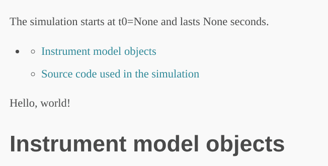
Among the many lines of text produced by the report, you can spot the presence of our «Hello, world!» message. Hurrah!

Let’s have a look at what happened. The first line imports the litebird_sim framework; since the name is quite long, it’s customary to shorten it to lbs:

import litebird_sim as lbs

The next interesting stuff happens when we instantiate a Simulation object:

sim = lbs.Simulation(base_path="./tut01")

Creating a Simulation object makes a lot of complicated things happen beyond the scenes. In this short example, what happens is the following:

1. The code checks if a directory named tut01 exists; if not, it is created.

2. An empty report is created.

The report is where the results of a simulation will be saved, and sections can be appended to it using the method Simulation.append_to_report(), like we did in our example:

sim.append_to_report("Hello, world!")

The report is actually written to disk only when Simulation.flush() is called:

sim.flush()

This is the most basic usage of the Simulation class; for more information, refer to Simulations.

In the next section, we will make something more interesting using the framework.

Interacting with the IMO

It’s not clear why we should want to install a whole framework just to create a HTML file, no matter how nice it looks. Things begin to get interesting once we start using other facilities provided by our framework.

Simulations for real-life experiments often require to use several parameters that describe the instruments being simulated: how many detectors there are, what are their properties, etc. These information are usually kept in an Instrument MOdel database, IMO for short.

The LiteBIRD IMO is managed using instrumentdb, a web-based database, but it can be retrieved also as a bundle of files. The LiteBIRD simulation framework seamlessy interacts with the IMO database and permits to retrieve all the parameters that describe the LiteBIRD instruments.

The best way to interact with the IMO is to have a local copy installed on your laptop. You should ask permission to the LiteBIRD Simulation Team for downloading the IMO from the (protected) site litebird_imo. Save it in a folder on your computer, e.g., /storage/litebird_imo, and then run the following command:

python -m litebird_sim.install_imo

and run the program interactively to configure the IMO. You typically want to use a «local copy»; specify the folder where the file schema.json you downloaded before resides (under /storage/litebird_imo in our case). Save the changes by pressing s, and you will have your IMO configured.

Our next example will use the IMO to run something more interesting:

import litebird_sim as lbs

sim = lbs.Simulation(base_path="./tut02")
lft_file = sim.imo.query(
    "/releases/v1.0/satellite/LFT/instrument_info"
)
sim.append_to_report(
    "The instrument {{ name }} has {{ num }} channels.",
    name=lft_file.metadata["name"],
    num=lft_file.metadata['number_of_channels'],
)
sim.flush()

If you run this program, it will produce a report containing the following message:

The instrument LFT has 12 channels.

Let’s dig into the code of the example. The first line looks almost the same as in the previous example:

# Previous example
sim = lbs.Simulation(base_path="./tut01")

# This example
sim = lbs.Simulation(base_path="./tut02")

Yet a big difference went unnoticed: since you configured the IMO using the install_imo module, the Simulation class managed to read the database contents and initialize a set of member variables. This is why we have been able to write the next line:

lft_file = sim.imo.query(
    "/releases/v1.0/satellite/LFT/instrument_info"
)

Although the parameter looks like a path to some file, it is a reference to a bit of information in the IMO; specifically, a set of parameters characterizing the instrument LFT (Low Frequency Telescope). This call retrieves the parameters and returns a DataFile object, which contains the information in its metadata field. These are used to fill the report:

sim.append_to_report(
    "The instrument {{ name }} has {{ num }} channels.",
    name=lft_file.metadata["name"],
    num=lft_file.metadata['number_of_channels'],
)

The code should be self-evident: the keywords name and num are used in the text to put some actual values within the placeholders {{ … }}. This is the syntax used by Jinja2, a powerful templating library.

This example showed you how to retrieve information from the IMO and introduced some features of the method Simulation.append_to_report(). To learn a bit more about the the IMO, read The Instrument Model Database (IMO); for reporting facilities, read Creating reports with litebird_sim.

Creating a coverage map

We’re now moving to something more «astrophysical»: we will write a program that computes the sky coverage of a scanning strategy over some time.

The code is complex because it uses several concepts explained in the section Scanning strategy; in fact, this example is very similar to the one shown in that section. It’s not needed that you understand everything, just have a look at the code that generates the report:

import litebird_sim as lbs
import healpy, numpy as np
import matplotlib.pylab as plt
import astropy.units as u

sim = lbs.Simulation(
    base_path="./tut04",
    start_time=0,
    duration_s=86400.,
)

sim.generate_spin2ecl_quaternions(
    scanning_strategy=lbs.SpinningScanningStrategy(
        spin_sun_angle_rad=np.deg2rad(30), # CORE-specific parameter
        spin_rate_hz=0.5 / 60,     # Ditto
        # We use astropy to convert the period (4 days) in
        # seconds
        precession_rate_hz=1.0 / (4 * u.day).to("s").value,
    )
)
instr = lbs.InstrumentInfo(
    name="core",
    spin_boresight_angle_rad=np.deg2rad(65),
)
det = lbs.DetectorInfo(name="foo", sampling_rate_hz=10)
obs, = sim.create_observations(detectors=[det])
pointings = obs.get_pointings(
    sim.spin2ecliptic_quats,
    detector_quats=[det.quat],
    bore2spin_quat=instr.bore2spin_quat,
)[0]

nside = 64
pixidx = healpy.ang2pix(nside, pointings[:, 0], pointings[:, 1])
m = np.zeros(healpy.nside2npix(nside))
m[pixidx] = 1
healpy.mollview(m)

sim.append_to_report("""

## Coverage map

Here is the coverage map:

![](coverage_map.png)

The fraction of sky covered is {{ seen }}/{{ total }} pixels
({{ "%.1f" | format(percentage) }}%).
""",
    figures=[(plt.gcf(), "coverage_map.png")],
    seen=len(m[m > 0]),
    total=len(m),
    percentage=100.0 * len(m[m > 0]) / len(m),
)

sim.flush()

This example is interesting because it shows how to interface Healpy with the report-generation facilities provided by our framework. As explained in Scanning strategy, the code above does the following things:

1. It generates a set of quaternions that encode the orientation of the spacecraft for the whole duration of the simulation (86,400 seconds, that is one day);

2. It creates an instance of the InstrumentInfo and DetectorInfo classes that represent a boresightdetector;

3. It generates a pointing information matrix;

4. It produces a coverage map by setting to 1 all those pixels that are visited by the directions encoded in the pointing information matrix.

Here is the part of the report containing the result:

The elements shown in this tutorial should allow you to generate more complex scripts. The next section detail the features of the framework in greater detail.